Generalized Linear Models#
Generalized Linear Models (GLMs) extend traditional linear regression by allowing for response variables that have different probability distributions. The relationship between predictors and response is established through a link function g(·):
Implementation Details
MoDeVa’s GLM implementation serves as a wrapper around scikit-learn’s linear models, providing:
Consistent API across all MoDeVa modeling frameworks
Direct access to scikit-learn’s robust implementations
Maintained compatibility with scikit-learn parameters
The underlying scikit-learn models include:
sklearn.linear_model.ElasticNet- Regularized regression with combined L1/L2 regularizationsklearn.linear_model.LogisticRegression- For classification tasks
All arguments available in scikit-learn’s API are preserved and can be passed directly through MoDeVa’s interface. This ensures users familiar with scikit-learn can leverage their existing knowledge while benefiting from MoDeVa’s enhanced interpretation capabilities.
GLM in MoDeVa#
Data Setup
from modeva import DataSet
# Create dataset object holder
ds = DataSet()
# Loading MoDeVa pre-loaded dataset "Bikesharing"
ds.load(name="BikeSharing")  # Changed dataset name
# Split data into training and testing sets randomly
ds.set_random_split()  # split the data into training and testing sets randomly
ds.set_target("cnt") # set the target variable
ds.scale_numerical(features=("cnt",), method="log1p") # scale the target variable
ds.preprocess() # preprocess the data
Model Setup
 from modeva.models import MoElasticNet, MoLogisticRegression

 # For regression tasks
model_glm = MoElasticNet(name="GLM",
                 feature_names=ds.feature_names, # feature names
                 feature_types=ds.feature_types, # feature types
                 alpha=0.01, # regularization parameter
                 l1_ratio = 0.5) # regularization parameter

 # For classification tasks
 model_glm = MoLogisticRegression(name="GLM",
                          feature_names=ds.feature_names, # feature names
                          feature_types=ds.feature_types) # feature types
For the full list of hyperparameters, please see the API of MoElasticNet and MoLogisticRegression.
Regularization Options
L1 Regularization
Controls sparsity
Helps with feature selection
L2 Regularization
Prevents overfitting
Stabilizes coefficients
Model Training
# train model with input: ds.train_x and target: ds.train_y
model_glm.fit(ds.train_x, ds.train_y)
Reporting and Diagnostics
# Create a testsuite that bundles dataset and model
from modeva import TestSuite
ts = TestSuite(ds, model_glm) # store bundle of dataset and model in fs
Performance Assessment
# View model performance metrics
result = ts.diagnose_accuracy_table()
# display the output
result.table
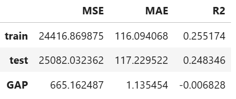
For the full list of arguments of the API see TestSuite.diagnose_accuracy_table.
Global Interpretation#
Regression Coefficients
View and interpret model coefficients:
# Plot coefficients all variables in the ds.feature_names
results = ts.interpret_coef(features=tuple(ds.feature_names))
results.plot()
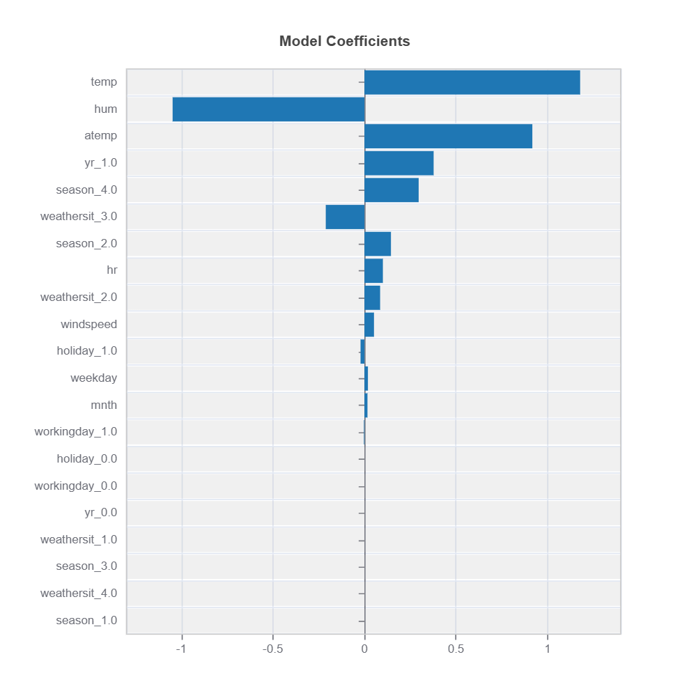
For the full list of arguments of the API see TestSuite.interpret_coef.
Key Aspects:
Positive coefficients indicate positive relationships
Negative coefficients indicate inverse relationships
Magnitude shows strength of relationship
Standardized features allow coefficient comparison
Feature Importance
Assess overall feature impact:
# Global feature importance
result = ts.interpret_fi()
# Plot the result
result.plot()
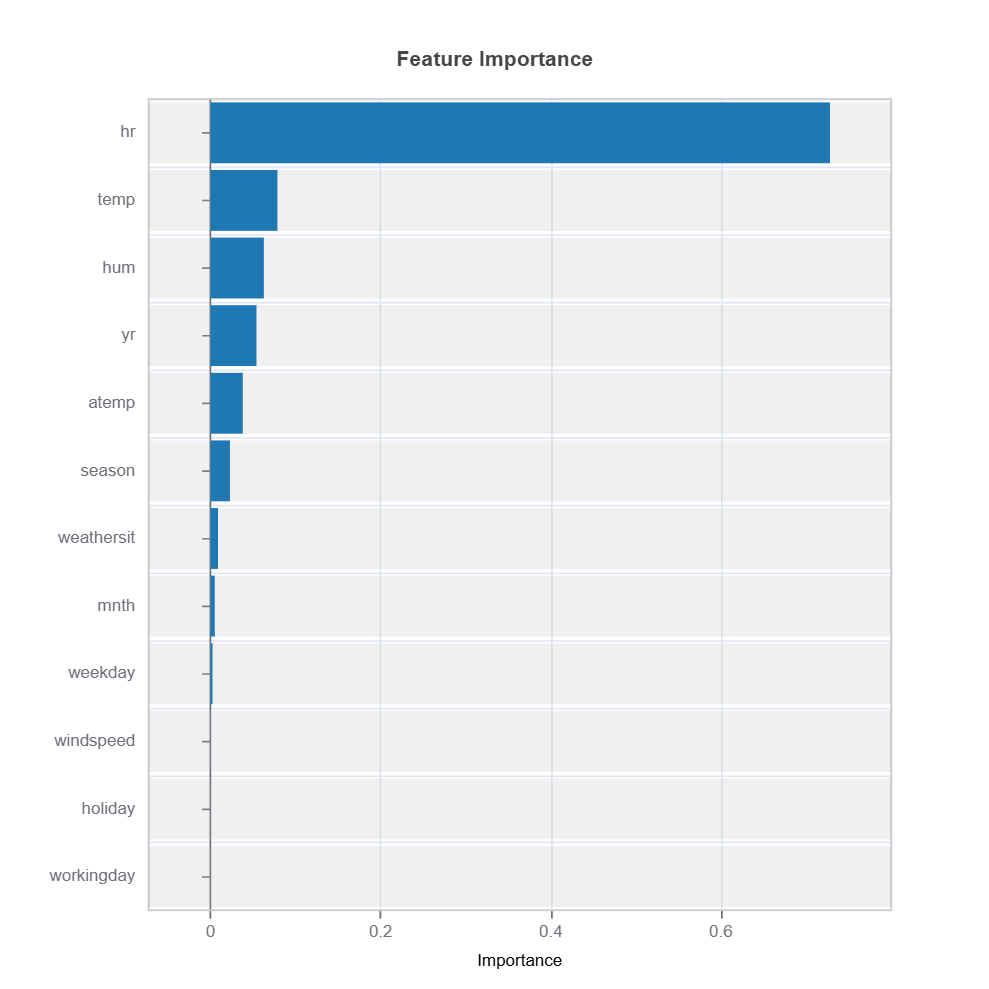
For the full list of arguments of the API see TestSuite.interpret_fi.
Importance Metrics:
Based on variance of marginal effects
Normalized to sum to 1
Higher values indicate stronger influence
Accounts for feature scale differences
Categorical Variables
One-hot encoded automatically
Can view importance per category
Interpretable through reference levels
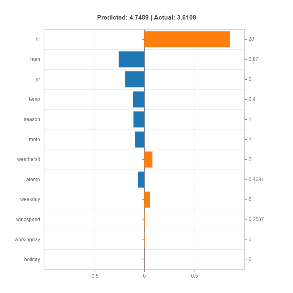
Local Interpretation#
Individual Prediction Analysis
# Local interpretation for specific sample: sample_index = 15
result = ts.interpret_local_fi(sample_index = 15, centered = True)
# Plot the result
result.plot()
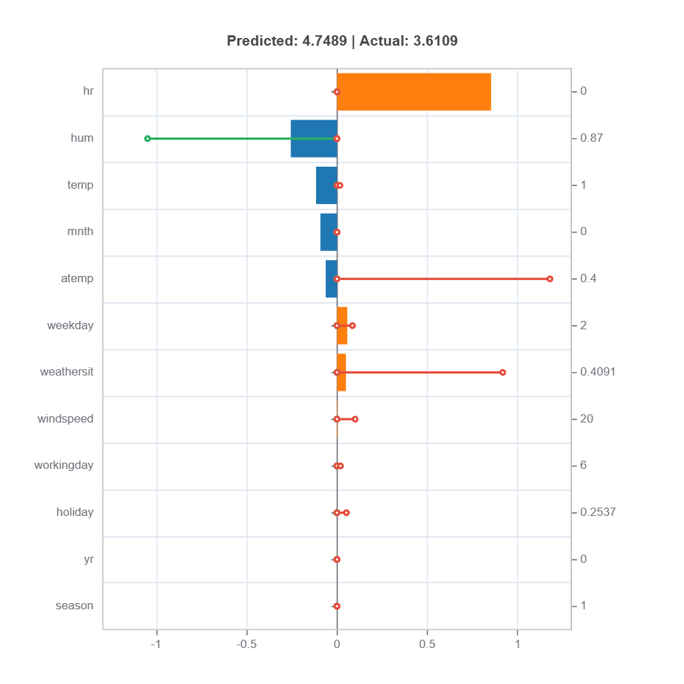
To show local importance along with regression coeficients:
# Local interpretation for specific sample: sample_index = 15
result = ts.interpret_local_linear_fi(sample_index = 15, centered = True)
# Plot the result
result.plot()
For the full list of arguments of the API see TestSuite.interpret_local_fi and TestSuite.interpret_local_linear_fi.
Components:
Stem: DIrection and magnitude to prediction (regression coefficient)
Bar: Direction and magnitude of effects (both coeffcient and feature value)
Feature values for the sample
Comparison to average behavior
Centering Options
Uncentered Analysis (centered=False):
Raw feature contributions
Direct interpretation
May have identifiability issues
Centered Analysis (centered=True):
Compares to population mean
More stable interpretation
Better for relative importance