Gradient Boosted Decision Trees

Gradient Boosted Decision Trees (GBDT) is a powerful ensemble learning algorithm that builds a sequence of decision trees, where each subsequent tree is trained to correct the errors of its predecessors. The algorithm works by iteratively fitting trees to the negative gradient of a loss function, enabling it to handle both regression and classification tasks with remarkable accuracy. Unlike random forests which build trees independently in parallel, GBDT constructs trees sequentially, with each tree learning from previous ones.

Mathematical Formulation

Overall Ensemble Model GBDT model can be written as sum of the initial model and the contributions of all the subsequent trees as follows:

\[F_M(x) = F_0(x) + \sum_{m=1}^M \gamma_m \cdot T_m(x)\]

where:

• \(F_0(x)\) is the initial model (often a constant value, such as the mean in regression tasks).

• \(T_m(x)\) is the decision tree (base learner) added at iteration

• \(\gamma_m\) is the learning rate (or step size) controlling the contribution of each tree.

• \(M\) is the total number of trees (iterations).

Pseudo-Residual Calculation At each iteration \(m\), the algorithm computes the pseudo-residuals, which are the negative gradients of the loss function \(L\) with respect to the current model’s predictions. For each sample \(x_i\) with true target \(y_i\), the pseudo-residual is given by:

\[r_{im} = -\left[\frac{\partial L(y_i, F(x_i))}{\partial F(x_i)}\right]{F(x) = F{m-1}(x)}\]

where:

• \(y_i\) is the true value for the \(i\) th sample.

• \(F_{m-1}(x_i)\) is the prediction for the \(i\) th sample after \(m-1\) iterations.

• \(r_{im}\) is the pseudo-residual for sample \(i\) at iteration \(m\)

Model Update After fitting a new decision tree \(h_m(x)\) to the pseudo-residuals, the model is updated as follows:

\[F_m(x) = F_{m-1}(x) + \gamma_m , h_m(x)\]

GBDT in MoDeVa

MoDeVa serves as a comprehensive wrapper around the leading GBDT implementations:

• XGBoost: Known for its speed and performance optimization

• LightGBM: Specializes in handling large-scale datasets efficiently

• CatBoost: Excels in processing categorical variables

The wrapper provides a unified interface while maintaining access to the underlying libraries’ specific capabilities and hyperparameters. This implementation choice ensures both ease of use and flexibility for advanced users.

Data Setup

from modeva import DataSet
## Create dataset object holder
ds = DataSet()
## Loading MoDeVa pre-loaded dataset "Bikesharing"
ds.load(name="BikeSharing")
## Preprocess the data
ds.scale_numerical(features=("cnt",), method="log1p") # Log transfomed target
ds.set_feature_type(feature="hr", feature_type="categorical") # set to categorical feature
ds.set_feature_type(feature="mnth", feature_type="categorical")
ds.scale_numerical(features=ds.feature_names_numerical, method="standardize") # standardized numerical features
ds.set_inactive_features(features=("yr", "season", "temp")) # deactivate some features
ds.preprocess()
## Split data into training and testing sets randomly
ds.set_random_split()

Model Setup

# For regression tasks using lightGBM, xgboost or catboost
from modeva.models import MoLGBMRegressor, MoXGBRegressor, MoCatBoostRegressor

# for lightGBM
model_gbdt = MoLGBMRegressor(name = "LGBM_model", max_depth=2, n_estimators=100)
# for xgboost
model_gbdt = MoXGBRegressor(name = "XGB_model", max_depth=2, n_estimators=100)
# for catboost
model_gbdt = MoCatBoostRegressor(name = "CBoost_model", max_depth=2, n_estimators=100)

# For classification tasks using lightGBM, xgboost or catboost
# for lightGBM
model_gbdt = MoLGBMClassifier(name = "LGBM_model", max_depth=2, n_estimators=100)
# for xgboost
model_gbdt = MoXGBClassifier(name = "XGB_model", max_depth=2, n_estimators=100)
# for catboost
model_gbdt = MoCatBoostClassifier(name = "CBoost_model", max_depth=2, n_estimators=100)

For the full list of hyperparameters, please see the API of

• LightGBM regressor and classifier: MoLGBMRegressor and MoLGBMClassifier.

• xgboost regressor and classifier: MoXGBRegressor and MoXGBClassifier.

• CatBoost regressor and classifier: MoCatBoostRegressor and MoCatBoostClassifier.

Model Training

# train model with input: ds.train_x and target: ds.train_y
model_gbdt.fit(ds.train_x, ds.train_y)

Reporting and Diagnostics

# Create a testsuite that bundles dataset and model
from modeva import TestSuite
ts = TestSuite(dataset, model_gbdt) # store bundle of dataset and model in fs

Performance Assessment

# View model performance metrics
result = ts.diagnose_accuracy_table()
# display the output
result.table

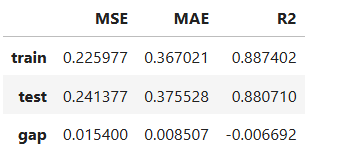
For the full list of arguments of the API see TestSuite.diagnose_accuracy_table.

Interpretability Through Functional ANOVA

While GBDT models are typically considered black boxes, they can be made interpretable through a functional ANOVA decomposition, particularly when tree depth is constrained. The functional ANOVA framework decomposes the model into additive components [Yang2024]:

\[f(x) = \mu + \sum _j f_j(x_j) + \sum_{j \lt k} f_{jk}(x_j, x_k) + ...\]

where:

• \(\mu\) is the global intercept

• \(f_j(x_j)\) represents main effects

• \(f_{jk}(x_j, x_k)\) represents interaction effects

Special Cases with Limited Depth

1. Depth-1 Trees (GAM Structure):

• Each tree makes a single split

• Results in a Generalized Additive Model (GAM)

• Model captures only main effects: \(f(x) = \mu + \sum_j f_j(x_j)\)

• Highly interpretable structure showing individual feature impacts

2. Depth-2 Trees (GAMI Structure):

• Each tree makes up to two splits

• Creates a GAM with Interactions (GAMI)

• Model captures both main effects and pairwise interactions: \(f(x) = \mu + \sum_j f_j(x_j) + \sum_{j<k} f_{jk}(x_j, x_k)\)

• Balances interpretability with ability to capture feature interactions

These constrained models offer several advantages:

• Maintain good predictive performance

• Provide clear interpretation of feature effects

• Enable visualization of feature relationships

• Support business decision-making with transparent logic

Functional ANOVA Decomposition Process for Tree Ensembles

1. Aggregation Stage

Base Representation

The tree ensemble model starts as a sum of tree structures:

\(f(x) = \sum_k \eta_k T_k(x)\)

where:

• \(k\) is the number of trees

• \(\eta_k\) are learning rates/weights

• \(T_k\) are individual trees

Leaf Node Decomposition

Each tree is rewritten as a sum of leaf nodes:

\(f(x) = \sum_m v_m \prod_j ∈ \sum_j I(s^l_{mj} \leq x_j \lt s^u_{mj})\)

where:

• \(m\) indexes leaf nodes

• \(v_m\) is leaf node value \(×\) tree weight

• \(S_m\) is the set of split variables in path to leaf \(m\)

• \([s^l_{mj}, s^u_{mj})\) defines interval for feature \(j\)

Effect Assignment

Leaf nodes are assigned to effects based on their distinct split variables:

1. Main Effects (1 split variable):

\(f_j(x_j) = \sum_{S_m=\{j\}} v_m · I(s^l_{mj} \leq x_j \lt s^u_{mj})\)

2. Pairwise Interactions (2 split variables):

\(f_{jk}(x_j,x_k) = \sum_{S_m=\{j,k\}} v_m · I(s^l_{mj} \leq x_j \lt s^u_{mj}) · I(s^l_{mk} \leq x_k \lt s^u_{mk})\)

3. Higher-order Interactions:

• Assigned based on number of distinct splits

• Maximum order limited by tree depth

2. Purification Stage

Identifiability Problem

Raw effects from aggregation may not have unique interpretation because:

• Main effects can be absorbed into parent interactions

• Multiple equivalent representations exist

• Effects may not be mutually orthogonal

Constraint Implementation

Effects must satisfy:

\(\int f_{i_1...i_t} x_{i_1},...,x_{i_t} \, dx_k = 0, k = i_1,...,i_t\)

and

\(\int f_{i_1...i_u} (x_{i_1},...,x_{i_u}) \, \cdot \, f_{j_1...j_v} (x_{j_1},...,x_{j_v}) \, d\mathbf{x} = 0, (i_1...i_u) \ne (j_1...j_v)\)

This ensures:

• All effects have zero means

• Effects are mutually orthogonal

Purification Algorithm

For a pairwise interaction \(f_{jk}(x_j,x_k):\)

1. First Dimension:

   • Calculate mean along \(x_j\) dimension

   • Subtract mean vector from interaction matrix

   • Add mean to main effect \(f_k(x_k)\)

2. Second Dimension:

   • Calculate mean along \(x_k\) dimension

   • Subtract mean vector from interaction matrix

   • Add mean to main effect \(f_j(x_j)\)

3. Iterate until convergence:

   • Repeat steps 1-2 until matrix change < threshold

   • Results in purified interaction and updated main effects

Cascade Process

1. Start with highest-order interactions

2. Recursively process lower-order effects

3. Finally center main effects

4. Add all removed means to intercept

Global Interpretation

The inherent interpretation of Depth-2 GBDT includes the main effect plot, pairwise interaction plot, effect importance plot, and feature importance plot.

Feature Importance

Assess overall feature impact:

# Global feature importance
result = ts.interpret_fi()
# Plot the result
result.plot()

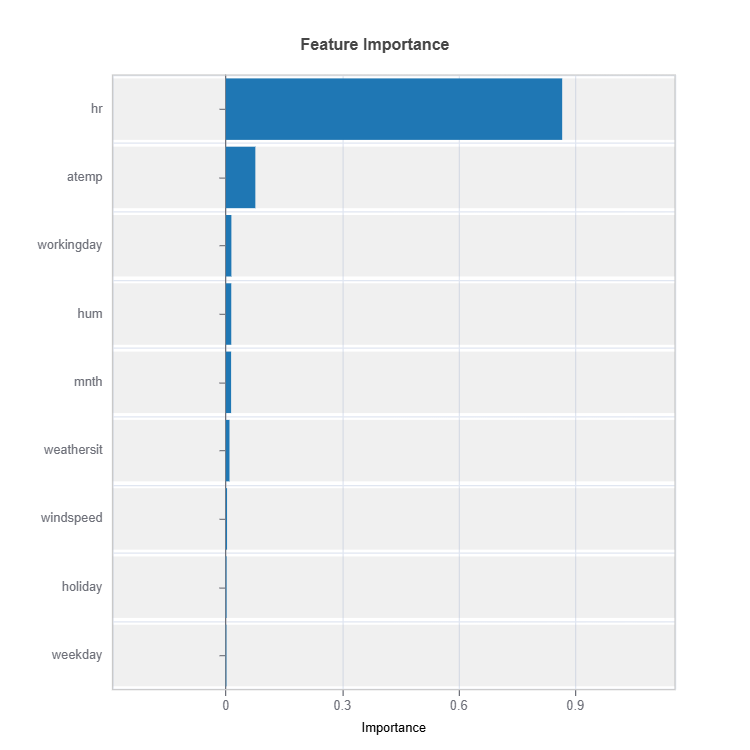
For the full list of arguments of the API see TestSuite.interpret_fi.

Importance Metrics:

• Based on variance of marginal effects

• Normalized to sum to 1

• Higher values indicate stronger influence

• Accounts for feature scale differences

Effect Importance

Assess overall impact according to functional ANOVA components: main and interaction effect

# Global effect importance
result = ts.interpret_ei()
# Plot the result
result.plot()

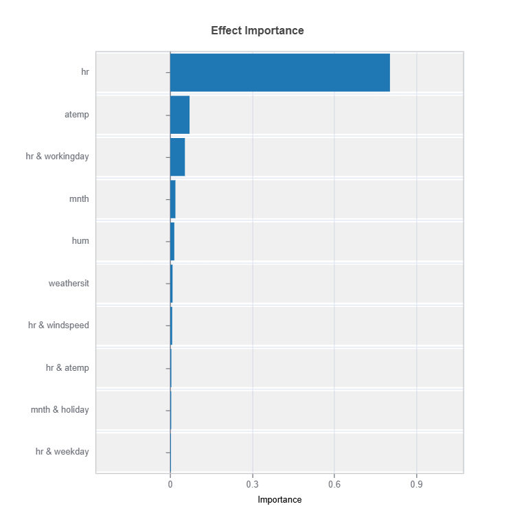
For the full list of arguments of the API see TestSuite.interpret_ei.

Importance Metrics:

• Based on variance of individual functional ANOVA term effects (main or interaction effect)

• Higher values indicate stronger influence

Categorical Variables

• One-hot encoded automatically

• Can view importance per category

• Interpretable through reference levels

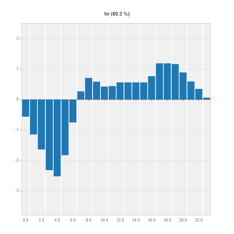
Global Effect Plot

Plot the main and interaction effect plot of features

# Main effect plot of feature: "hr"
result = ts.interpret_effects(features = "hr")
# Plot the result
result.plot()

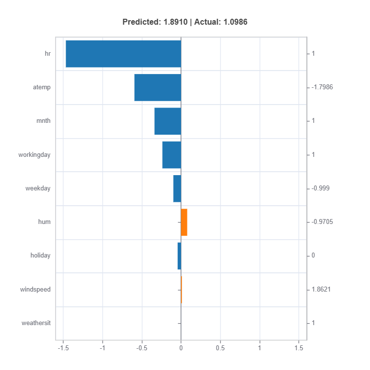
Local Interpretation

Individual Prediction Analysis

# Local interpretation for specific sample: sample_index = 10
result = ts.interpret_local_fi(sample_index = 10, centered = True)   # local feature importance
# Plot the result
result.plot()

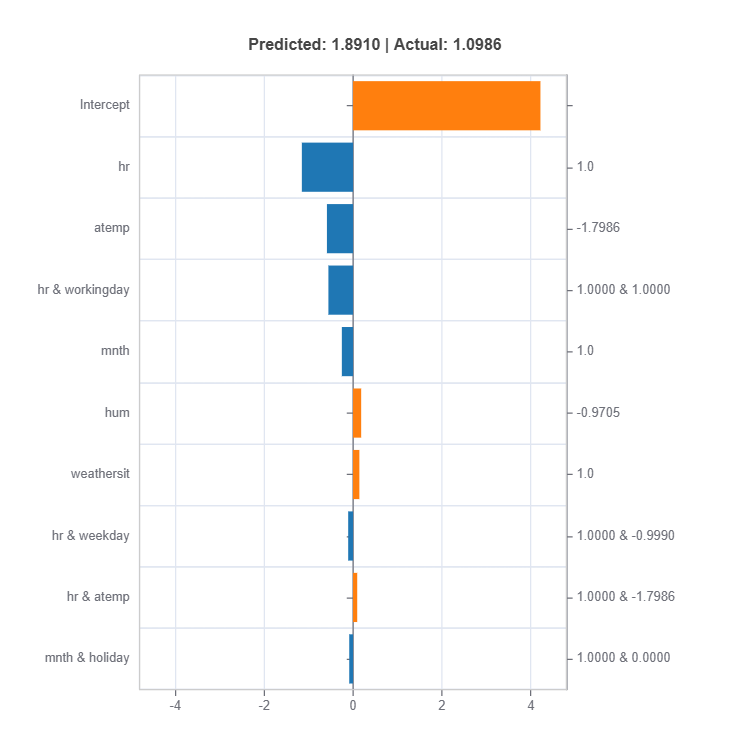
result = ts.interpret_local_ei(sample_index = 10, centered = True)   # local effect importance
# Plot the result
result.plot()

For the full list of arguments of the API see TestSuite.interpret_local_fi and TestSuite.interpret_local_ei .

Components:

• Feature or Effect contributions to prediction

• Feature or Effect values for the sample

• Comparison to average behavior

• Direction and magnitude of effects

Centering Options

1. Uncentered Analysis (centered=False): * Raw feature contributions * Direct interpretation * May have identifiability issues

2. Centered Analysis (centered=True): * Compares to population mean * More stable interpretation * Better for relative importance

Monotonicity Constraint in GBDT

Monotonicity constraints are essential in many real-world applications where certain feature-response relationships must follow domain knowledge. For example:

• Credit scoring should increase with income

• Risk should decrease with credit rating

• Property value should increase with square footage

xgboost regressor and classifier: MoXGBRegressor and MoXGBClassifier provide ability to control monotonicity.

Benefits

Interpretability Enhancement

1. Shape Functions

• Smoother main effects

• Reduced noise and fluctuations

• Clearer global patterns

2. Local Explanations

• More consistent SHAP values

• Easier to explain individual predictions

• Better aligned with business logic

Model Quality

1. Robustness

• Reduced overfitting

• Better generalization

• More reliable extrapolation

2. Performance

• Often maintains or improves accuracy

• More stable predictions

• Better handling of sparse regions

Interaction with ANOVA Decomposition

Main Effects

• Guarantees monotonic shape for constrained features

• Preserves interpretability in functional decomposition

• Simplifies effect visualization

Pairwise Interactions

• Maintains partial monotonicity

• More interpretable interaction patterns

• Cleaner effect separation

Empirical Results

1. Monotonicity constraints often lead to minimal performance loss

2. Significant improvement in interpretability metrics

3. Better generalization in some cases

4. More reliable predictions in sparse data regions

Examples

Example 1: Bike Sharing

The example below demonstrates how to use MoDeVa with its high-code APis for the Bike Sharing dataset from the UCI repository, which consists of 20,640 samples and 9 features, fetched by sklearn.datasets. The response variable MedHouseVal (Median Home Value) is continuous and is a regression problem.

• Tree Ensemble Models (Regression)

Examples 2: Taiwan Credit

The second example below demonstrates how to use MoDeVa’s high-code APIs for the TaiwanCredit dataset from the UCI repository. This dataset comprises the credit card details of 30,000 clients in Taiwan from April 2005 to September 2005, and more information can be found on the TaiwanCreditData website. The FlagDefault variable serves as the response for this classification problem.

• Tree Ensemble Models (Classification)

References

References

[Yang2024]

Zebin Yang, Agus Sudjianto, Xiaoming Li and Aijun Zhang (2024). Inherently Interpretable Tree Ensemble Learning, arXiv preprint arXiv:2410.19098.