Neural Tree#
The Neural Tree model is an extension of Gradient Boosted Linear Trees (GBLT). It converts the discrete (hard) splits of a traditional GBLT into continuous (soft) splits by employing a sigmoid function. This transformation renders the model fully differentiable and enables end-to-end training using backpropagation. In practice, the Neural Tree is initialized with parameters obtained from a pre-trained GBLT, which are then fine-tuned to potentially improve predictive performance and robustness.
The architecture provides an inherently interpretable model through functional ANOVA decomposition while maintaining the predictive power of tree ensembles.
Model architecture#
The overall prediction function of the Neural Tree ensemble is given by:
where:
\(\mathbf{x} = (x_1, x_2, \dots, x_d)\) denotes the feature vector.
\(f_0\) is the baseline prediction (e.g., the global mean).
\(\gamma_m\) is the weight associated with the \(m\) th tree.
\(T_m(\mathbf{x})\) is the differentiable tree function of the :math:mth Neural Tree.
Each Neural Tree \(T_m(\mathbf{x})\) follows the structure of a depth‑1 linear tree from GBLT, but with soft (differentiable) splits. Specifically, the tree output is computed as a blend of two terminal linear models:
Soft Split Function: The split is made differentiable by replacing the hard decision with a sigmoid function:
where:
\(\sigma(z) = \frac{1}{1 + e^{-z}}\) is the sigmoid function.
\(x_{j_m}\) is the feature chosen for splitting in tree \(m\).
\(t_m\) is the threshold parameter.
\(a_m\) controls the steepness of the sigmoid (i.e., the softness of the split).
Terminal Linear Models: Each branch of the tree has a linear model that computes its prediction. The outputs for the left and right branches are:
where \(\beta_{m0}^{(L)}\), \(\beta_{mi}^{(L)}\) and \(\beta_{m0}^{(R)}\), \(\beta_{mi}^{(R)}\) are the intercepts and coefficients of the linear models in the left and right branches, respectively.
The output of the \(m\) th Neural Tree is then given by:
Training Process The training of the Neural Tree model involves two main stages:
Initialization with GBLT: A standard Gradient Boosted Linear Tree model is first trained using conventional methods. Its parameters – including the split feature \(x_{j_m}\), threshold \(t_m\), terminal linear model coefficients, and tree weights \(\gamma_m\) – are then used to initialize the Neural Tree.
Refinement via Backpropagation: With the hard splits replaced by differentiable soft splits, the entire model becomes end-to-end differentiable. The model is subsequently refined using gradient-based optimization (backpropagation) to further optimize all parameters (including \(a_m\), \(t_m\), the linear coefficients, and \(\gamma_m\) which are the weights of final layers in Neural Networks).
Neural Tree in MoDeVa#
Data Setup
from modeva import DataSet
## Create dataset object holder
ds = DataSet()
## Loading MoDeVa pre-loaded dataset "Bikesharing"
ds.load(name="BikeSharing")
## Preprocess the data
ds.scale_numerical(features=("cnt",), method="log1p") # Log transfomed target
ds.set_feature_type(feature="hr", feature_type="categorical") # set to categorical feature
ds.set_feature_type(feature="mnth", feature_type="categorical")
ds.scale_numerical(features=ds.feature_names_numerical, method="standardize") # standardized numerical features
ds.set_inactive_features(features=("yr", "season", "temp")) # deactivate some features
ds.preprocess()
## Split data into training and testing sets randomly
ds.set_random_split()
Model Setup
# For regression tasks
from modeva.models import MoNeuralTreeRegressor
model_neut = MoNeuralTreeRegressor(name="NeuralTree", n_estimators=100)

# For classification tasks
from modeva.models import MoNeuralTreeClassifier
model_neut = MoNeuralTreeClassifier(name = "NeuralTree", n_estimators=100)
For the full list of hyperparameters, please see the API of MoNeuralTreeRegressor and MoNeuralTreeClassifier.
Model Training
# train model with input: ds.train_x and target: ds.train_y
model_neut.fit(ds.train_x, ds.train_y)
Reporting and Diagnostics Setup
# Create a testsuite that bundles dataset and model
from modeva import TestSuite
ts = TestSuite(ds, model_neut) # store bundle of dataset and model in fs
Performance Assessment
# View model performance metrics
result = ts.diagnose_accuracy_table()
# display the output
result.table
For the full list of arguments of the API see TestSuite.diagnose_accuracy_table.
Functional ANOVA Representation#
For interpretability, the overall prediction function \(f(\mathbf{x})\) can be decomposed into additive components using a functional ANOVA framework as follows:
The decomposition is defined as follows:
Baseline:
Main Effects: For each feature \(x_i\):
where \(\mathbf{x}_{\setminus i}\) denotes all features except \(x_i\).
Interaction Effects: For each feature pair \((x_i, x_j)\):
This decomposition isolates the contributions of individual features and their interactions, aiding in model interpretability.
See the aggregation and purification process for Gradient Boosted Decision Trees <https://modeva.ai/_build/html/_source/user_guide/models/gbdt.html>.
Step-by-Step Process#
1. Initialize with GBLT: Train a Gradient Boosted Linear Tree model to obtain initial parameters: Splitting feature \(x_{j_m}\), threshold \(t_m\), and initial linear model coefficients. Tree weights \(\gamma_m\).
2. Convert Hard Splits to Soft Splits: Replace the hard threshold with a soft split using:
3. Compute Neural Tree Output: Calculate the output of each Neural Tree:
4. Aggregate the Ensemble: Form the overall prediction:
5. Refine via Backpropagation: Optimize all parameters of the Neural Tree (including \(a_m\), \(t_m\), the terminal model coefficients, and \(\gamma_m\)) using gradient descent.
6. Apply Functional ANOVA: Decompose \(f(\mathbf{x})\) into baseline, main effects, and interaction effects to gain interpretability.
See the aggregation and purification process for Gradient Boosted Decision Trees <https://modeva.ai/_build/html/_source/user_guide/models/gbdt.html>.
Effect Attribution#
1. Local Effect Attribution:
Main effect contribution: \(f_j(x_j)\)
Interaction contribution: \(f_{jk}(x_j, x_k)\)
2. Feature Attribution:
\[z_j(x_j) = f_j(x_j) + \frac{1}{2} \sum_k f_{jk}(x_j, x_k)\]
Global Interpretation#
The inherent interpretation of NeuralTree includes the main effect plot, pairwise interaction plot, effect importance plot, and feature importance plot.
Feature Importance#
Assess overall feature impact:
# Global feature importance
result = ts.interpret_fi()
# Plot the result
result.plot()
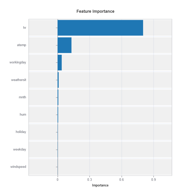
For the full list of arguments of the API see TestSuite.interpret_fi.
Importance Metrics:
Based on variance of marginal effects
Normalized to sum to 1
Higher values indicate stronger influence
Accounts for feature scale differences
Effect Importance#
Assess overall impact according to functional ANOVA components: main and interaction effect
# Global effect importance
result = ts.interpret_ei()
# Plot the result
result.plot()
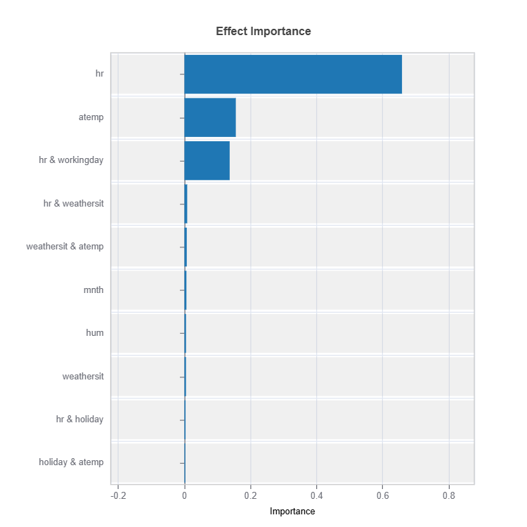
For the full list of arguments of the API see TestSuite.interpret_ei.
Importance Metrics:
Based on variance of individual functional ANOVA term effects (main or interaction effect)
Higher values indicate stronger influence
Categorical Variables
One-hot encoded automatically
Can view importance per category
Interpretable through reference levels
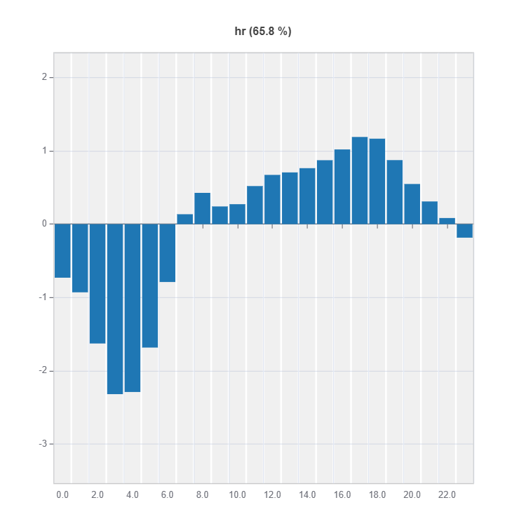
Global Effect Plot#
Plot the main and interaction effect plot of features
# Main effect plot of feature: "hr"
result = ts.interpret_effects(features = "hr")
# Plot the result
result.plot()
# Interaction effect plot of features: "hr" and "workingday"
result = ts.interpret_effects(features = ("hr","workingday"))
# Plot the result
result.plot()
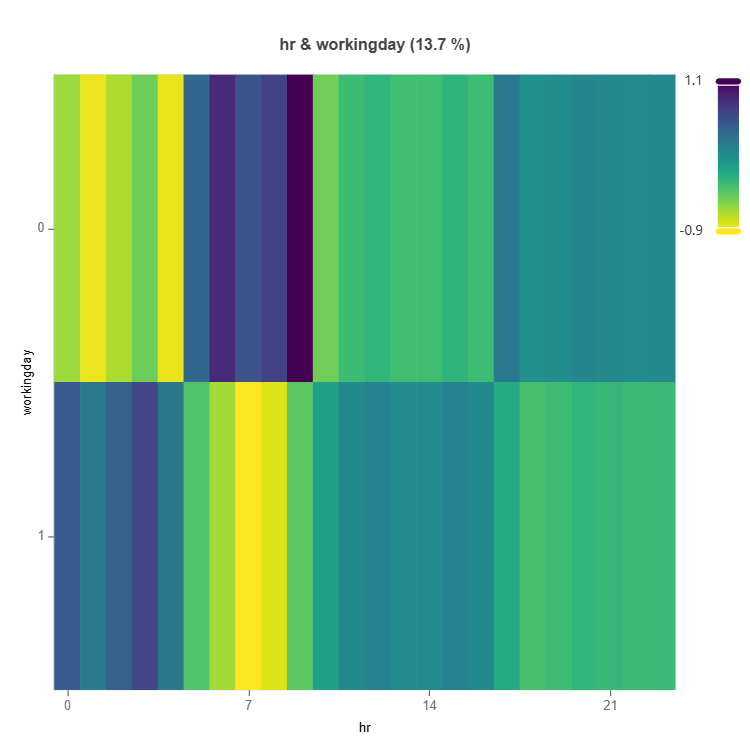
For the full list of arguments of the API see TestSuite.interpret_effects.
Local Interpretation#
Individual Prediction Analysis#
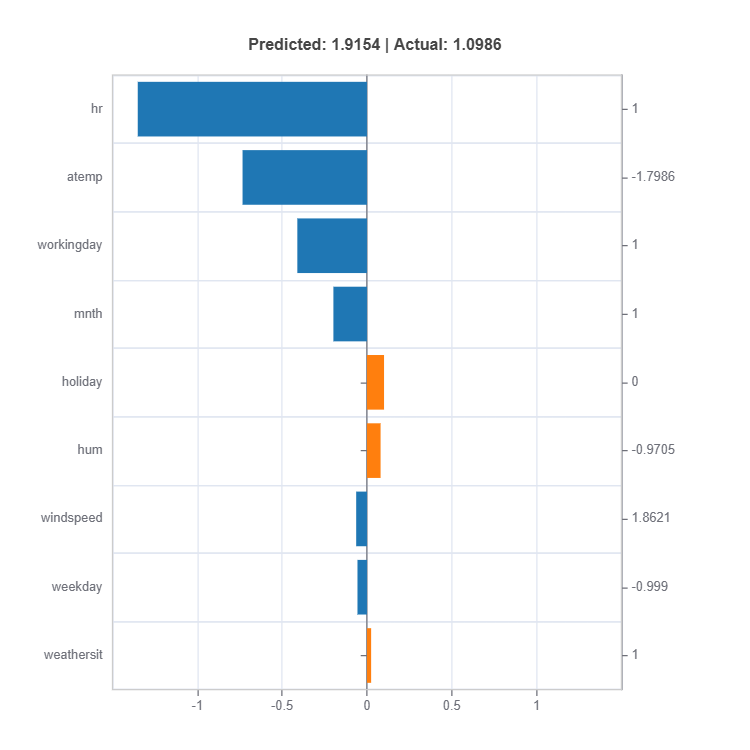
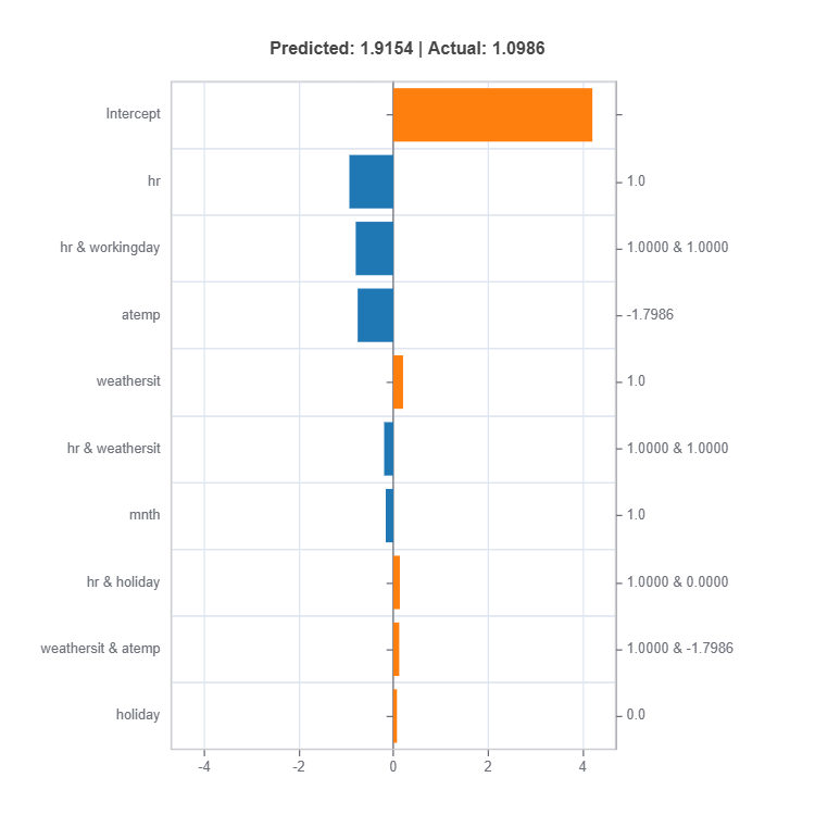
# Local interpretation for specific sample: sample_index = 10
result = ts.interpret_local_fi(sample_index = 10, centered = True)   # local feature importance
# Plot the result
result.plot()
result = ts.interpret_local_ei(sample_index = 10, centered = True)   # local effect importance
# Plot the result
result.plot()
For the full list of arguments of the API see TestSuite.interpret_local_fi and TestSuite.interpret_local_ei .
Components:
Feature or Effect contributions to prediction
Feature or Effect values for the sample
Comparison to average behavior
Direction and magnitude of effects
Centering Options
Uncentered Analysis (centered=False):
Raw feature contributions
Direct interpretation
May have identifiability issues
Centered Analysis (centered=True):
Compares to population mean
More stable interpretation
Better for relative importance
Monotonicity Constraints in Neural Tree#
Enforcing monotonicity constraints to align with domain knowledge is often nneded to ensure model conceptual soundness. In many applications where GAMI-Net is deployed, certain input features should have a consistently positive or negative effect on predictions:
In credit scoring, higher income should lead to better credit ratings
In medical risk assessment, increased risk factors should result in higher risk scores
In pricing models, larger product quantities should correspond to higher total costs
While NeuralTree structure provides natural interpretability, explicitly enforcing monotonicity makes the model more reliable and trustworthy. Without monotonicity constraints, even interpretable models may learn relationships that violate logical domain constraints, particularly in regions with sparse training data.
Loss Function with Monotonicity Constraint#
Neural Tree augments its standard loss function with a monotonicity constraint penalty that operates on both main effects and interaction terms:
where:
\(l(\theta)\) is the base prediction loss
\(\gamma\) is the monotonicity penalty coefficient
\(M\) is the set of features that should be monotonic
\(\frac{\partial \hat{y}}{\partial x_i}\) is the gradient of prediction with respect to feature i
Explanation
The loss function has three components working together to create an interpretable and conceptually sound model:
The prediction loss \(l(\theta)\) ensures accurate predictions.
The monotonicity penalty \(\max(0, -\frac{\partial \hat{y}}{\partial x_i})^2\) enforces monotonic relationships for specified features by penalizing negative gradients.
This formulation is particularly powerful in NeuralTree because it enforces monotonicity while preserving the model’s structure. The monotonicity constraints apply to both individual feature effects and their interactions, ensuring that the entire model respects domain knowledge about feature relationships.
The strength of monotonicity enforcement can be tuned through \(\gamma\), allowing practitioners to balance between strict monotonicity and prediction accuracy. When \(\gamma\) is large, the model will strongly enforce monotonicity even if it means slightly reduced accuracy. When \(\gamma\) is smaller, the model has more flexibility to fit the data while still maintaining some monotonic tendency.
Implementation Considerations#
When implementing monotonicity constraints in GAMI-Net:
Provide the lists of input variables that have monotonically increasing and decreasing in the API: mono_increasing_list=(), mono_decreasing_list=()
Start with a small monotonic regularization reg_mono and gradually increase it until desired monotonicity is achieved
NeuralTree is using sampling with sample size controlled by `mono_sample_size`to check monotonicity
Evaluate both prediction performance and monotonicity violations
Verify monotonicity holds for both main effects and interaction terms
Consider using validation data to tune the reg_mono parameter