Linear Tree and Gradient Boosted Linear Trees

Linear Tree

Linear Trees aim to combine the strengths of traditional decision trees with the power of linear models.

Basic Concept

• Traditional Decision Trees: Use constant predictions at their leaves. For example, in regression tasks, each leaf simply predicts the mean value of the target variable for the data points falling into that leaf.

• Linear Trees:Enhance this by replacing the constant value at the leaves with a linear model. Each leaf contains a small regression model that predicts the target as a linear combination of the features specific to that leaf. This allows the model to:

  • Handle local linear trends in the data.

  • Introduce flexibility to capture non-linear relationships through tree splits.

  • For certain data type, it can provide better predictive performance than constant-leaf decision trees for problems with local linearity.

Model Structure

\[\begin{split}f(x) = \begin{cases} \beta_1^\mathrm{T}x + \alpha_1 & \text{if } x \text{ follows path to leaf 1}\\ \beta_2^\mathrm{T}x + \alpha_2 & \text{if } x \text{ follows path to leaf 2}\\ \vdots & \vdots\\ \beta_L^\mathrm{T}x + \alpha_L & \text{if } x \text{ follows path to leaf L} \end{cases}\end{split}\]

Linear Tree in MoDeVa

Data Setup

from modeva import DataSet
## Create dataset object holder
ds = DataSet()
## Loading MoDeVa pre-loaded dataset "Bikesharing"
ds.load(name="BikeSharing")
## Preprocess the data
ds.scale_numerical(features=("cnt",), method="log1p") # Log transfomed target
ds.set_feature_type(feature="hr", feature_type="categorical") # set to categorical feature
ds.set_feature_type(feature="mnth", feature_type="categorical")
ds.scale_numerical(features=ds.feature_names_numerical, method="standardize") # standardized numerical features
ds.set_inactive_features(features=("yr", "season", "temp")) # deactivate some features
ds.preprocess()
## Split data into training and testing sets randomly
ds.set_random_split()

Model Setup

# For regression tasks
from modeva.models import MoGLMTreeRegressor
model_glmt = MoGLMTreeRegressor(name="GLMT", max_depth=10)

# For classification tasks
from modeva.models import MoGLMTreeClassifier
model_glmt = MoGLMTreeBoostClassifier(name = "GLMT", max_depth=10)

For the full list of hyperparameters, please see the API of MoGLMTreeRegressor and MoGLMTreeClassifier.

Model Training

# train model with input: ds.train_x and target: ds.train_y
model_glmt.fit(ds.train_x, ds.train_y)

Reporting and Diagnostics

# Create a testsuite that bundles dataset and model
from modeva import TestSuite
ts = TestSuite(dataset, model_glmt) # store bundle of dataset and model in fs

Performance Assessment

# View model performance metrics
result = ts.diagnose_accuracy_table()
# display the output
result.table

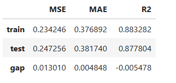
For the full list of arguments of the API see TestSuite.diagnose_accuracy_table.

Advantages

Local Flexibility:

• Captures more nuanced patterns in the data because the linear model in each leaf can adapt to local trends.

• Improved Predictive Power: Compared to traditional decision trees, linear trees reduce bias in regions where the target variable has linear relationships with input features.

• Interpretable: Each leaf’s linear model can provide insight into the feature contributions for predictions in that region.

Gradient Boosted Linear Tree (GBLT)

Algorithm

• Extends gradient boosting framework

• Uses Linear Trees as base learners [Hu2023]

• Sequential ensemble building

Training Process

1. Initialize model with a constant value

2. For each iteration:

   • Compute residuals/gradients

   • Fit Linear Tree to them

   • Update ensemble

Model Formulation

A boosted ensemble where each tree \(T_m\) is a depth‑1 (decision stump) model that assigns a linear prediction at its terminal nodes. The overall boosted model is given by

\[f(\mathbf{x}) = f_0 + \sum_{m=1}^M \gamma_m \, T_m(\mathbf{x}),\]

where:

• \(\mathbf{x} = (x_1, x_2, \dots, x_d)\) is the feature vector.

• \(f_0\) is the baseline (e.g., the global mean).

• \(\gamma_m\) is the weight for the \(m\) th tree.

• \(T_m(\mathbf{x})\) is the prediction function of tree \(m\).

Tree Structure \(T_m\)

Each tree \(T_m\) performs a split on a selected feature \(x_{j_m}\) at threshold \(t_m\) and applies a linear model in each of the two regions. That is,

\[\begin{split}T_m(\mathbf{x}) = \begin{cases} \beta_{m0}^{(L)} + \displaystyle\sum_{i=1}^d \beta_{mi}^{(L)}\, x_i, & \text{if } x_{j_m} \le t_m, \\[1em] \beta_{m0}^{(R)} + \displaystyle\sum_{i=1}^d \beta_{mi}^{(R)}\, x_i, & \text{if } x_{j_m} > t_m. \end{cases}\end{split}\]

Here:

• \(\beta_{m0}^{(L)}\) and \(\beta_{m0}^{(R)}\) are the intercepts for the left and right nodes.

• \(\beta_{mi}^{(L)}\) and \(\beta_{mi}^{(R)}\) are the coefficients for feature \(x_i\) in the left and right terminal nodes, respectively.

Overall Model \(f(\mathbf{x})\)

The boosted model aggregates the contributions from all trees:

\[f(\mathbf{x}) = f_0 + \sum_{m=1}^M \gamma_m \, T_m(\mathbf{x}).\]

GBLT in MoDeVa

Model Setup

# For regression tasks
from modeva.models import MoGLMTreeBoostRegressor
model_gblt = MoGLMTreeBoostRegressor(name="GBLT", max_depth=1, n_estimators=100)

# For classification tasks
from modeva.models import MoGLMTreeBoostClassifier
model_gblt = MoGLMTreeBoostClassifier(name = "GBLT", max_depth=1, n_estimators=100)

For the full list of hyperparameters, please see the API of MoGLMTreeBoostRegressor and MoGLMTreeBoostClassifier.

Model Training

# train model with input: ds.train_x and target: ds.train_y
model_gblt.fit(ds.train_x, ds.train_y)

Reporting and Diagnostics Setup

# Create a testsuite that bundles dataset and model
from modeva import TestSuite
ts = TestSuite(ds, model_gblt) # store bundle of dataset and model in fs

Performance Assessment

# View model performance metrics
result = ts.diagnose_accuracy_table()
# display the output
result.table

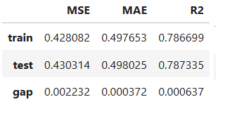
For the full list of arguments of the API see TestSuite.diagnose_accuracy_table.

Functional ANOVA Decomposition

The goal is to decompose \(f(\mathbf{x})\) into additive components that represent the baseline, main effects, and interaction effects:

\[f(\mathbf{x}) = f_0 + \sum_{i=1}^d f_i(x_i) + \sum_{1 \le i < j \le d} f_{ij}(x_i, x_j) + \cdots\]

The components are defined as follows:

• Baseline:

  \[f_0 = \mathbb{E}[f(\mathbf{x})].\]

• Main Effects: For each feature \(x_i\),

  \[f_i(x_i) = \mathbb{E}_{\mathbf{x}_{\setminus i}} \bigl[ f(\mathbf{x}) \mid x_i \bigr] - f_0,\]

  where \(\mathbf{x}_{\setminus i}\) denotes all features except \(x_i:math:\).

• Interaction Effects: For each pair \((x_i, x_j)\),

  \[f_{ij}(x_i, x_j) = \mathbb{E}_{\mathbf{x}_{\setminus \{i,j\}}} \bigl[ f(\mathbf{x}) \mid x_i, x_j \bigr] - f_i(x_i) - f_j(x_j) - f_0.\]

See the aggregation and purification process for Gradient Boosted Decision Trees <https://modeva.ai/_build/html/_source/user_guide/models/gbdt.html>.

Step-by-Step Transformation

1. Train the Boosted Ensemble: Build the model using LightGBM with depth‑1 trees. For each tree \(T_m\), record:

   • The splitting feature \(x_{j_m}\) and threshold \(t_m\).

   • The linear models for each terminal node:

     • For \(x_{j_m} \le t_m\):

       \[T_m^{(L)}(\mathbf{x}) = \beta_{m0}^{(L)} + \sum_{i=1}^d \beta_{mi}^{(L)}\, x_i.\]

     • For \(x_{j_m} > t_m\):

       \[T_m^{(R)}(\mathbf{x}) = \beta_{m0}^{(R)} + \sum_{i=1}^d \beta_{mi}^{(R)}\, x_i.\]

2. Aggregate Tree Predictions: Combine the trees to form the overall prediction function:

   \[f(\mathbf{x}) = f_0 + \sum_{m=1}^M \gamma_m \, T_m(\mathbf{x}).\]

3. Compute the Baseline \(f_0\) : Determine the overall mean prediction:

   \[f_0 = \mathbb{E}[f(\mathbf{x})].\]

4. Derive Main Effects \(f_i(x_i)\): For each feature \(x_i:math:\), calculate its main effect by averaging over the remaining features:

   \[f_i(x_i) = \mathbb{E}_{\mathbf{x}_{\setminus i}} \bigl[ f(x_i, \mathbf{x}_{\setminus i}) \bigr] - f_0.\]

5. Extract Interaction Effects \(f_{ij}(x_i, x_j)\): For every pair of features, compute the joint effect and subtract the main effects and baseline:

   \[f_{ij}(x_i, x_j) = \mathbb{E}_{\mathbf{x}_{\setminus \{i,j\}}} \bigl[ f(x_i, x_j, \mathbf{x}_{\setminus \{i,j\}}) \bigr] - f_i(x_i) - f_j(x_j) - f_0.\]

6. Interpret and Visualize: Use the resulting decomposition to:

   • Visualize the individual main effects \(f_i(x_i)\) (e.g., line plots).

   • Plot the interaction effects \(f_{ij}(x_i, x_j)\) (e.g., heatmaps or surface plots).

   • Gain insights into which features or interactions drive the predictions and assess the model’s robustness.

Global Interpretation

The inherent interpretation of GAMI-Net includes the main effect plot, pairwise interaction plot, effect importance plot, and feature importance plot.

Feature Importance

Assess overall feature impact:

# Global feature importance
result = ts.interpret_fi()
# Plot the result
result.plot()

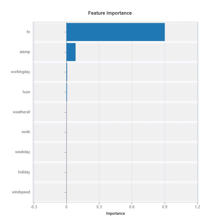
For the full list of arguments of the API see TestSuite.interpret_fi.

Importance Metrics:

• Based on variance of marginal effects

• Normalized to sum to 1

• Higher values indicate stronger influence

• Accounts for feature scale differences

Effect Importance

Assess overall impact according to functional ANOVA components: main and interaction effect

# Global effect importance
result = ts.interpret_ei()
# Plot the result
result.plot()

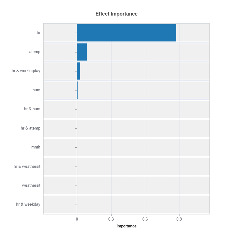
For the full list of arguments of the API see TestSuite.interpret_ei.

Importance Metrics:

• Based on variance of individual functional ANOVA term effects (main or interaction effect)

• Higher values indicate stronger influence

Categorical Variables

• One-hot encoded automatically

• Can view importance per category

• Interpretable through reference levels

Global Effect Plot

Plot the main and interaction effect plot of features

# Main effect plot of feature: "hr"
result = ts.interpret_effects(features = "hr")
# Plot the result
result.plot()

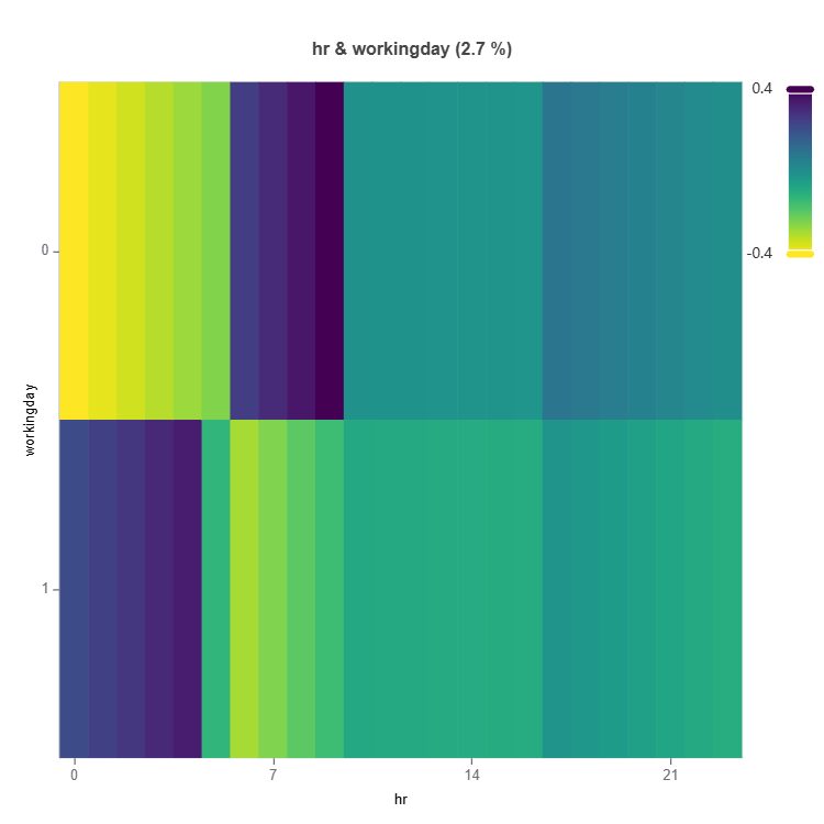
For the full list of arguments of the API see TestSuite.interpret_effects.

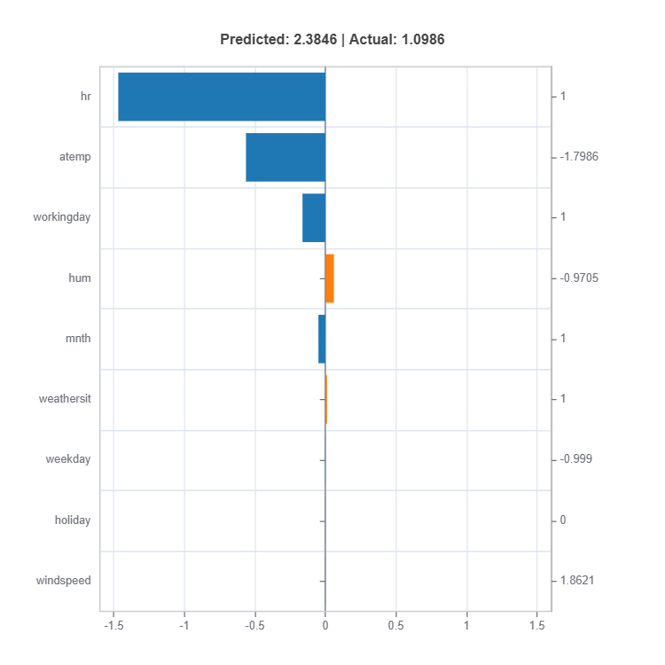
Local Interpretation

Individual Prediction Analysis

# Local interpretation for specific sample: sample_index = 10
result = ts.interpret_local_fi(sample_index = 10, centered = True)   # local feature importance
# Plot the result
result.plot()

result = ts.interpret_local_ei(sample_index = 10, centered = True)   # local effect importance
# Plot the result
result.plot()

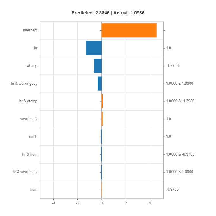
For the full list of arguments of the API see TestSuite.interpret_local_fi and TestSuite.interpret_local_ei .

Components:

• Feature or Effect contributions to prediction

• Feature or Effect values for the sample

• Comparison to average behavior

• Direction and magnitude of effects

Centering Options

1. Uncentered Analysis (centered=False):

   • Raw feature contributions

   • Direct interpretation

   • May have identifiability issues

2. Centered Analysis (centered=True):

   • Compares to population mean

   • More stable interpretation

   • Better for relative importance

Examples

Example 1: Bike Sharing

The example below demonstrates how to use MoDeVa with its high-code APis for the Bike Sharing dataset from the UCI repository, which consists of 20,640 samples and 9 features, fetched by sklearn.datasets. The response variable MedHouseVal (Median Home Value) is continuous and is a regression problem.

• Linear Tree Regression

Examples 2: Taiwan Credit

The second example below demonstrates how to use MoDeVa’s high-code APIs for the TaiwanCredit dataset from the UCI repository. This dataset comprises the credit card details of 30,000 clients in Taiwan from April 2005 to September 2005, and more information can be found on the TaiwanCreditData website. The FlagDefault variable serves as the response for this classification problem.

• Linear Tree Classification

References

References

[Hu2023]

Linwei Hu, Vijayan N. Nair, Agus Sudjianto, Aijun Zhang and Jie Chen (2024). Interpretable Machine Learning based on Functional ANOVA Framework: Algorithms and Comparisons, arXiv preprint arXiv:2305.15670.