Mixture of Experts (MoE)

Modern datasets—whether in finance, healthcare, or marketing—are inherently heterogeneous, comprising multiple subpopulations with distinct characteristics and drivers. Traditional “one-size-fits-all” models often fall short in such settings, leading to suboptimal predictions and reduced robustness when faced with shifts in data distribution. This motivates the need for advanced modeling approaches that achieve the following objectives:

Capturing Data Heterogeneity: By adaptively learning both local and global patterns, a model can tailor its predictions to the nuanced behaviors within different regions of the data. This adaptive learning not only improves overall predictive accuracy but also facilitates a deeper understanding of the complex interactions present in diverse datasets.

Segmented Models with Actionable Insights: Many real-world applications benefit from identifying and modeling distinct segments within the data, as each segment may be driven by unique factors. Segmenting the data enables the development of specialized models that highlight the critical drivers for each subgroup, thereby supporting targeted decision-making and interpretable results.

Enhanced Resilience Against Distribution Drift: A mixture of experts (MoE) framework naturally supports more homogeneous performance across varying data segments. By training specialized experts on segments that share similar characteristics, the model is less vulnerable to distribution drift. This segmentation ensures that even if one part of the data distribution shifts, the corresponding expert remains well-calibrated, thereby enhancing the overall model’s robustness and stability.

To address these challenges, MoDeVa provides a mixture of experts model that integrates soft clustering with expert predictors. Initially, the data is partitioned into clusters, with each sample receiving a probabilistic membership assignment across clusters. Specialized XGBoost models are then trained for each cluster using weighted samples, and their predictions are aggregated based on these membership probabilities. Furthermore, the cluster centroids are optimized via Particle Swarm Optimization (PSO), dynamically refining the segmentation to ensure that both local expertise and global patterns are effectively captured.

This approach not only enhances predictive performance by accommodating data heterogeneity and uncovering distinct drivers but also delivers more resilient and uniformly performing models in the face of distribution drift.

The Mixture of Experts (MoE) model in MoDeVa combines multiple interpretable XGBoost models, each specializing in different regions of the feature space. By using shallow trees (depth 1 or 2) for both gating and expert models, it maintains interpretability through functional ANOVA decomposition while enabling local expertise development.

Key Benefits:

• Interpretable predictions

• Local specialization

• Robust performance

• Clear effect attribution

Model Architecture

The model consists of three main components:

1. Gating Model:

• Determines cluster memberships

• Assigns sample weights

2. Expert Models:

• Individual XGBoost models

• Depth-restricted trees

3. Mixture Layer:

• Combines expert predictions

• Weights by membership probabilities

• Produces final output

Mathematical Formulation

Given a dataset \(\mathcal{D} = {(x_i, y_i)}_{i=1}^n\) where \(x_i \in \mathbb{R}^d\) represents the feature vector and \(y_i\) is the target, the model employs \(K\) experts. Each expert \(f_k(x)\) is an XGBoost model, and the overall prediction is a weighted combination of the experts’ outputs.

Soft Membership Calculation For each data point \(x_i\) and cluster \(k\) with centroid \(c_k\), the probability membership is computed using a softmax over the negative squared Euclidean distance scaled by a temperature parameter \(\tau\):

(1)\[p_{ik} = \frac{\exp\left(-\frac{|x_i - c_k|^2}{\tau}\right)} {\sum_{j=1}^K \exp\left(-\frac{|x_i - c_j|^2}{\tau}\right)}\]

Expert Prediction Aggregation Each expert \(f_k(x)\) is trained on the full dataset with samples weighted by their respective membership \(p_{ik}\). The aggregated prediction for an input \(x\) is given by:

(2)\[\hat{y}(x) = \sum_{k=1}^K p_k(x) . f_k(x)\]

Overall Loss Function The model’s parameters, which include the experts’ parameters \(\theta\) and the cluster centroids \({c_k}_{k=1}^K\), are optimized by minimizing the loss function:

(3)\[L(\theta, {c_k}) = \sum_{i=1}^n \ell\Bigl(y_i, \hat{y}(x_i)\Bigr)\]

Here, \(\ell\) denotes an appropriate loss function (e.g., squared error for regression or log-loss for classification).

Centroid Optimization via Particle Swarm Optimization (PSO) Due to the non-differentiability of XGBoost, the cluster centroids are optimized using Particle Swarm Optimization (PSO). In PSO, each particle represents a candidate set of centroids, and the particle updates are defined as follows:

PSO Velocity Update Equation

(4)\[v_{i}^{(t+1)} = \omega\, v_{i}^{(t)} + c_1\, r_1\, \Bigl(p_{i,\text{best}} - x_{i}^{(t)}\Bigr) + c_2\, r_2\, \Bigl(g_{\text{best}} - x_{i}^{(t)}\Bigr)\]

PSO Position Update Equation

(5)\[x_{i}^{(t+1)} = x_{i}^{(t)} + v_{i}^{(t+1)}\]

Step-by-Step Process

Initialization:

• Define \(K\): Select the number of clusters/experts.

• Centroid Initialization: Initialize the cluster centroids \({c_k}_{k=1}^K\) using a clustering method such as k-means.

• PSO Setup: Initialize a swarm of particles, where each particle represents a candidate set of centroids. Set initial velocities and PSO parameters ( \(\omega\), \(c_1\), and \(c_2\)).

Soft Assignment:

For each data point \(x_i\), compute the soft membership probabilities \(p_{ik}\) using Equation (1).

Expert Training:

Train an XGBoost model \(f_k(x)\) for each cluster \(k\). Each training sample is weighted by its corresponding membership \(p_{ik}\) to focus the expert on its relevant data region.

Prediction Aggregation:

For a given input \(x\), compute the membership probabilities \(p_k(x)\) and obtain the overall prediction using Equation (2).

Loss Computation:

Evaluate the overall loss \(L(\theta, {c_k})\) across the dataset as per Equation (3).

Centroid Optimization via PSO:

• Particle Evaluation: For each particle (candidate centroids), update the soft assignments, retrain the experts as necessary, and compute the overall loss.

• Particle Update: Update the velocities and positions of the particles using Equations (4) and (5).

• Selection: Choose the particle with the lowest loss as the best candidate.

• Iteration: Repeat the PSO process until the loss converges or a maximum number of iterations is reached.

Iteration and Convergence:

Iterate the entire process by recomputing soft assignments, retraining experts, and re-optimizing centroids until the model performance stabilizes.

MoE in MoDeVa

Data Setup

from modeva import DataSet
## Create dataset object holder
ds = DataSet()
## Loading MoDeVa pre-loaded dataset "Bikesharing"
ds.load(name="BikeSharing")
## Preprocess the data
ds.scale_numerical(features=("cnt",), method="log1p") # Log transfomed target
ds.set_feature_type(feature="hr", feature_type="categorical") # set to categorical feature
ds.set_feature_type(feature="mnth", feature_type="categorical")
ds.scale_numerical(features=ds.feature_names_numerical, method="standardize") # standardized numerical features
ds.set_inactive_features(features=("yr", "season", "temp")) # deactivate some features
ds.preprocess()
## Split data into training and testing sets randomly
ds.set_random_split()

Model Setup

# For regression tasks
from modeva.models import MoMoERegressor
model_moe = MoMoERegressor(name="MOE_Regression", max_depth=2, n_clusters=2, n_estimators=100)

# For classification tasks
from modeva.models import MoMoEClassifier
model_moe = MoMoEClassifier("MOE_Classification", max_depth=2, n_clusters=2, n_estimators=100)

For the full list of hyperparameters, please see the API of MoMoERegressor and MoMoEClassifier.

Model Training

# train model with input: ds.train_x and target: ds.train_y
model_moe.fit(ds.train_x, ds.train_y)

Reporting and Diagnostics Setup

# Create a testsuite that bundles dataset and model
from modeva import TestSuite
ts = TestSuite(ds, model_moe) # store bundle of dataset and model in fs

Performance Assessment

# View model performance metrics
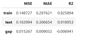
result = ts.diagnose_accuracy_table()
# display the output
result.table

Interpretation: Functional ANOVA Representation

Model interpretation is attributed to its individual expert model and functional ANOVA decomposition is similar to that of Gradient Boosted Decision Tree

Gating Decomposition

The gating model decomposes as:

\[p_j(x) = \mu_j + \sum_i g_{ij}(x_i) + \sum_{ik} g_{ikj}(x_i, x_k)\]

where:

• \(\mu_j\) is base membership probability

• \(g_{ij}(x_i)\) are main effects

• \(g_{ikj}(x_i, x_k)\) are interaction effects

Expert Decomposition

Each expert model decomposes as:

\[f_j(x) = \mu_j + \sum_i f_{ij}(x_i) + \sum_{ik} f_{ikj}(x_i, x_k)\]

where:

• \(\mu_j\) is expert’s base prediction

• \(f_{ij}(x_i)\) are expert’s main effects

• \(f_{ikj}(x_i, x_k)\) are expert’s interactions

Effect Attribution

Local effects are computed for:

1. Gating Model:

   • Feature contributions to memberships (probability membership/weight)

   • Region assignments

2. Expert Models:

   • Feature effects on predictions

   • Interaction patterns

   • Local behavior

Global Interpretation

The inherent interpretation of GAMI-Net includes the main effect plot, pairwise interaction plot, effect importance plot, and feature importance plot.

Feature Importance

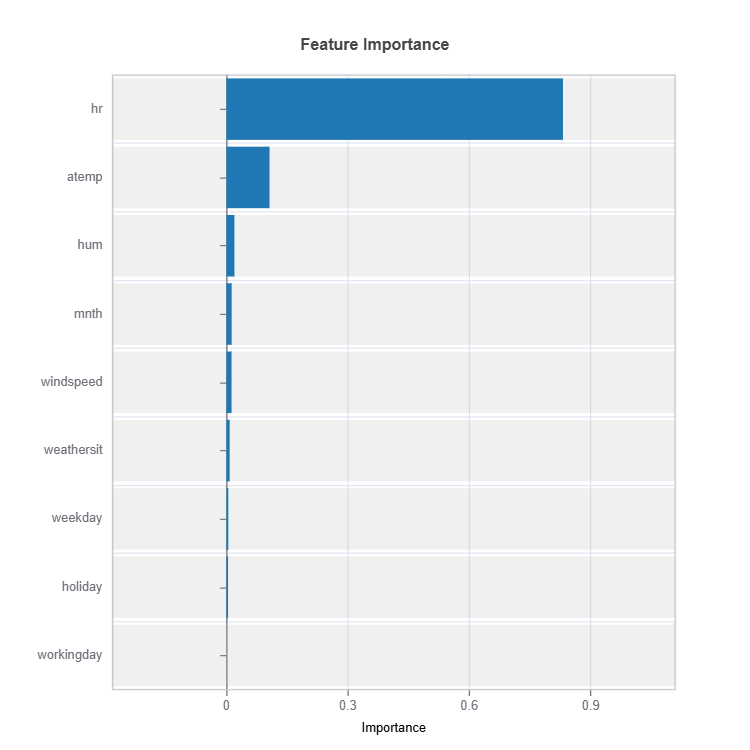
Feature impacts in MoE are calculated for each cluster (expert).

# Global feature importance
result = ts.interpret_fi()
# Plot the result
result.plot()

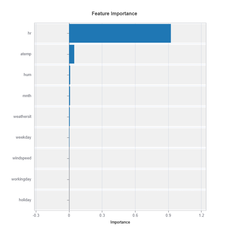
Feature important plots will be generated for each cluster (expert). The following are some examples.

For the full list of arguments of the API see TestSuite.interpret_fi.

Importance Metrics:

• Based on variance of marginal effects

• Normalized to sum to 1

• Higher values indicate stronger influence

• Accounts for feature scale differences

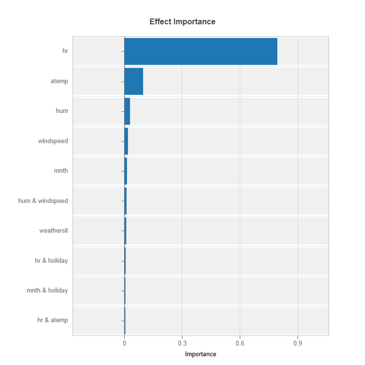
Effect Importance

Impact according to functional ANOVA components (main and interaction effects) are calculated for each cluster (expert)

# Global effect importance
result = ts.interpret_ei()
# Plot the result
result.plot(n_bars = 10) # Only top 10 are displayed

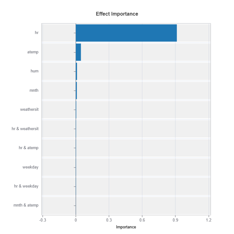
For the full list of arguments of the API see TestSuite.interpret_ei.

Importance Metrics:

• Based on variance of individual functional ANOVA term effects (main or interaction effect)

• Higher values indicate stronger influence

Categorical Variables

• One-hot encoded automatically

• Can view importance per category

• Interpretable through reference levels

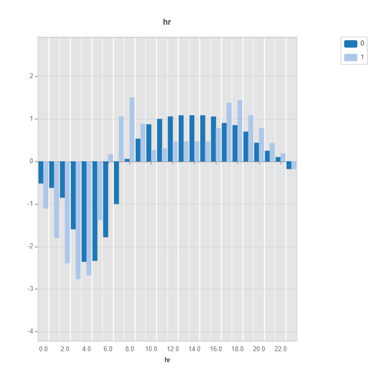
Global Effect Plot

Plot the main and interaction effect plot of features for each cluster (expert)

# Main effect plot of feature: "hr"
result = ts.interpret_effects(features = "hr")
# Plot the result
result.plot()

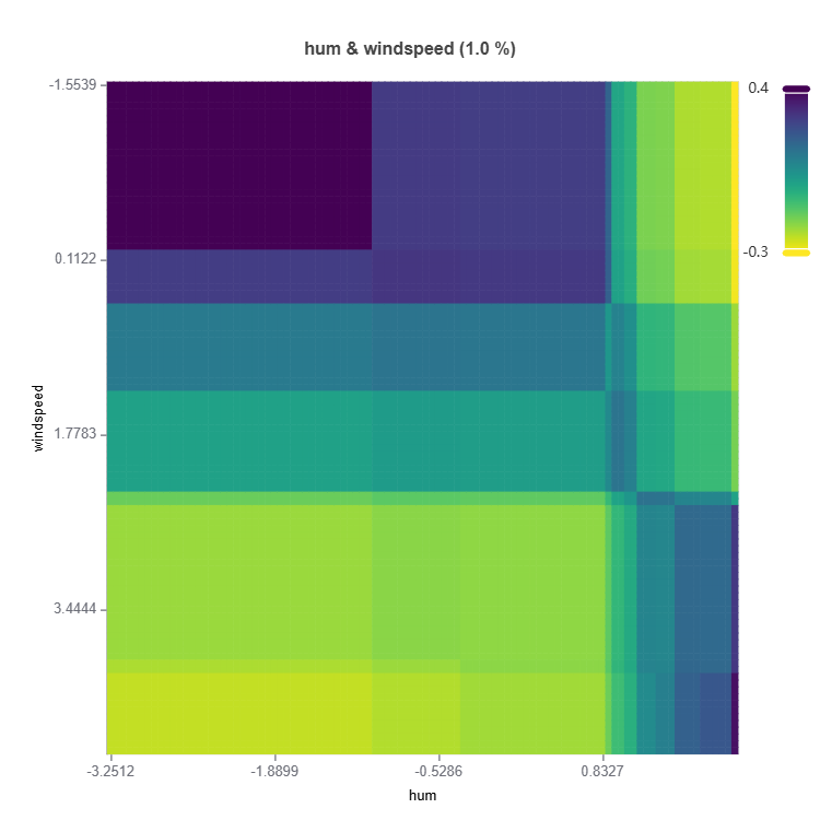
# Interaction effect plot of features: "hum" and "windspeed"
result = ts.interpret_effects(features = ("hum","windspeed"))
# Plot the result
result.plot()

To plot specific expert use:

# Main effect plot of feature: "hr"
result = ts.interpret_effects(features = "hr")
expert_name = "0" # expert name/number to plot
result.plot(expert_name)

To plot all experts to compare:

# Main effect plot of feature: "hr"
result = ts.interpret_effects(features = "hr")
expert_no = "0" # expert number to plot
result.plot(name = "all")

For the full list of arguments of the API see TestSuite.interpret_effects.

Local Interpretation

Local interpretation is calculated for each cluster (expert).

Individual Prediction Analysis

# Local interpretation for specific sample: sample_index = 10
result = ts.interpret_local_fi(sample_index = 10, centered = True)   # local feature importance
# Plot the result
result.plot()

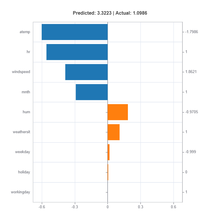
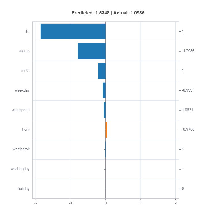
The local feature importances for each cluster (expert) for sample number 10.

result = ts.interpret_local_ei(sample_index = 10)   # local effect importance
# Plot the result
result.plot(n_bars = 10)

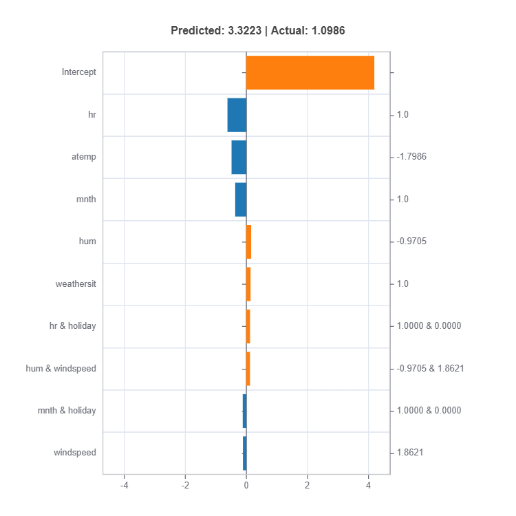
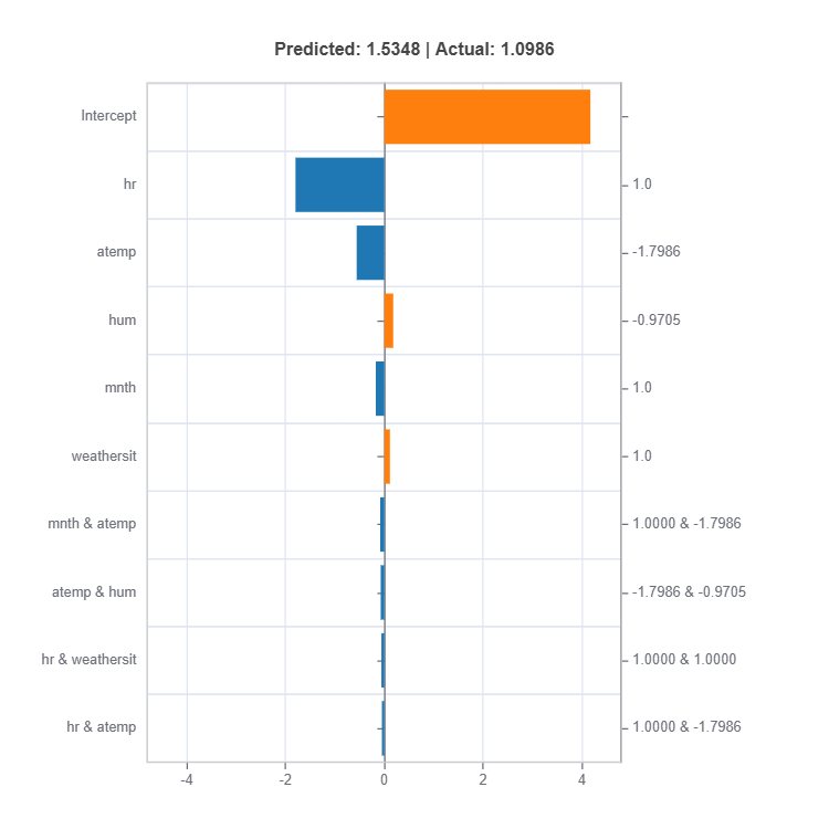
The local feature importances for each cluster (expert) for sample number 10.

For the full list of arguments of the API see TestSuite.interpret_local_fi and TestSuite.interpret_local_ei .

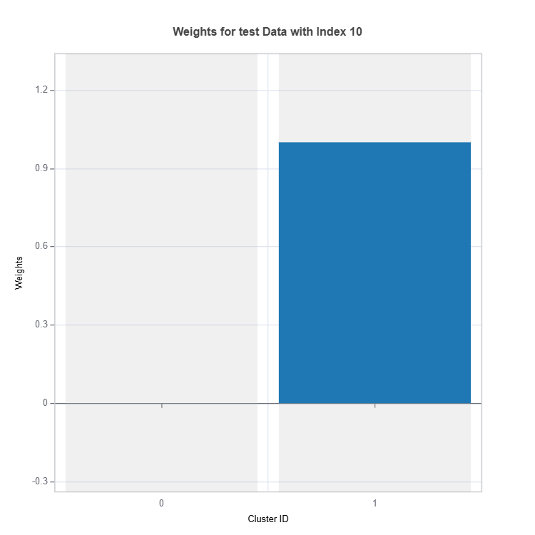
The weights (contribution) of experts to overall response can be checked as follows:

results = ts.interpret_local_moe_weights(sample_index = 10)
results.plot()

For the full list of arguments of the API see `TestSuite.interpret_local_moe_weights`_

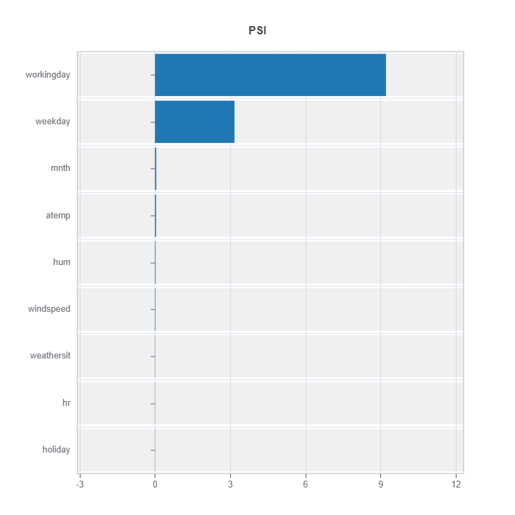
To understand the distribution difference between a cluster (expert) to the rest, marginal distribution distance such as using PSI can be displayed as follows.

results = ts.interpret_moe_cluster_analysis()
cluster_no = 2
data_results = ds.data_drift_test(**results.value[cluster_no]["data_info"],
                               distance_metric="PSI",
                               psi_method="uniform",
                               psi_bins=10)
data_results.plot("summary")

For the full list of arguments of the API see DataSet.data_drift_test.

Examples

Example 1: Bike Sharing

The example below demonstrates how to use MoDeVa with its high-code APis for the Bike Sharing dataset from the UCI repository, which consists of 20,640 samples and 9 features, fetched by sklearn.datasets. The response variable MedHouseVal (Median Home Value) is continuous and is a regression problem.

• Mixture of Expert (MoE) Regression

Examples 2: Taiwan Credit

The second example below demonstrates how to use MoDeVa’s high-code APIs for the TaiwanCredit dataset from the UCI repository. This dataset comprises the credit card details of 30,000 clients in Taiwan from April 2005 to September 2005, and more information can be found on the TaiwanCreditData website. The FlagDefault variable serves as the response for this classification problem.

• Mixture of Expert (MoE) Classification