GAMI-Net

GAMI-Net (Generalized Additive Models with Structured Interactions Network) is an explainable neural network architecture designed to balance prediction accuracy with interpretability [Yang2020]. It builds on traditional Generalized Additive Models (GAMs) by incorporating structured pairwise interactions while maintaining interpretability through these constraints:

• Sparsity: Selects only significant effects for a parsimonious model.

• Heredity: Includes interaction terms only if at least one parent main effect exists.

• Marginal Clarity: Distinguishes between main effects and interactions.

GAMI-Net employs a disentangled feedforward network with separate subnetworks for main effects and pairwise interactions. These are visualized via 1D line plots and 2D heatmaps. It is flexible enough to handle numerical and categorical variables, offering competitive predictive performance with high interpretability.

Model Structure

• Main Effects: Captured in individual subnetworks.

• Pairwise Interactions: Identified and modeled in separate subnetworks.

• Monotonicity (Optional): Ensures features follow a specific increasing or decreasing pattern via regularization.

\[\begin{align} g(\mathbb{E}(y|\textbf{x})) = \mu + \sum\limits_{j} h_{j}(x_{j}) + \sum\limits_{j<k} f_{jk}(x_{j},x_{k}), \tag{1} \end{align}\]

Training Process

1. Train Main Effects: Learn and prune trivial main effect subnetworks.

2. Model Pairwise Interactions:

   • Identify candidate interactions using heredity constraints.

   • Evaluate interaction importance using FAST scoring.

   • Train top-K interaction subnetworks and prune trivial ones.

3. Fine-Tune: Retrain all components (main effects and interactions) simultaneously.

Compared to tree-based models, GAMI-Net has a continuous and smooth shape function, which is more interpretable. Also, it is very flexible to incorporate various interpretability constraints in neural networks.

GAMI-Net in MoDeVa

Data Setup

## Create dataset object holder
ds = DataSet()
## Loading MoDeVa pre-loaded dataset "Bikesharing"
ds.load(name="BikeSharing")
## Preprocess the data
ds.scale_numerical(features=("cnt",), method="log1p") # Log transfomed target
ds.scale_numerical(features=ds.feature_names, method="standardize") # standardized numerical features
ds.set_inactive_features(features=("yr", "season", "temp")) # deactivate some features
ds.preprocess()
## Split data into training and testing sets randomly
ds.set_random_split()

Model Setup

# For regression tasks
from modeva.models import MoGAMINetRegressor
model_GAMI = MoGAMINetRegressor()

# For classification tasks
from modeva.models import MoReLUDNNClassifier
model_GAMI = MoGAMINetClassifier(max_epochs=(100, 100, 100))

For the full list of hyperparameters, please see the API of MoGAMINetRegressor and MoGAMINetClassifier.

Model Training

# train model with input: ds.train_x and target: ds.train_y
model_GAMI.fit(ds.train_x, ds.train_y.ravel())

Reporting and Diagnostics

# Create a testsuite that bundles dataset and model
from modeva import TestSuite
ts = TestSuite(ds, model_GAMI) # store bundle of dataset and model in fs

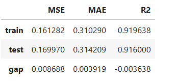
Performance Assessment

# View model performance metrics
result = ts.diagnose_accuracy_table()
# display the output
result.table

Functional ANOVA Representation

Basic Decomposition

The model decomposes into additive components:

\[f(x) = \mu + \sum _j f_j(x_j) + \sum_{j<k} f_{jk}(x_j, x_k)\]

where:

• \(\mu\) is the global intercept

• \(f_j(x_j)\) represents main effects

• \(f_{jk}(x_j, x_k)\) represents pairwise interaction effects

Effect Computation

For interpretability, the overall prediction function \(f(\mathbf{x})\) can be decomposed into additive components using a functional ANOVA framework as follows:

\[f(\mathbf{x}) = f_0 + \sum_{i=1}^d f_i(x_i) + \sum_{1 \le i < j \le d} f_{ij}(x_i, x_j) + \cdots\]

The decomposition is defined as follows:

Baseline:

\[f_0 = \mathbb{E}[f(\mathbf{x})].\]

Main Effects: For each feature \(x_i\):

\[f_i(x_i) = \mathbb{E}{\mathbf{x}{\setminus i}} \bigl[ f(\mathbf{x}) \mid x_i \bigr] - f_0,\]

where \(\mathbf{x}_{\setminus i}\) denotes all features except \(x_i\).

Interaction Effects: For each feature pair \((x_i, x_j)\):

\[f_{ij}(x_i, x_j) = \mathbb{E}{\mathbf{x}{\setminus {i,j}}} \bigl[ f(\mathbf{x}) \mid x_i, x_j \bigr] - f_i(x_i) - f_j(x_j) - f_0.\]

This decomposition isolates the contributions of individual features and their interactions, aiding in model interpretability.

Purification Constraints

1. Zero Mean:

   \[\int f_{i_1...i_t} x_{i_1},...,x_{i_t} \, dx_k = 0, k = i_1,...,i_t\]

2. Orthogonality:

   \[\int f_{i_1...i_u} (x_{i_1},...,x_{i_u}) \, \cdot \, f_{j_1...j_v} (x_{j_1},...,x_{j_v}) \, d\mathbf{x} = 0, (i_1...i_u) \ne (j_1...j_v)\]

See the aggregation and purification process for Gradient Boosted Decision Trees <https://modeva.ai/_build/html/_source/user_guide/models/gbdt.html>.

Effect Attribution

1. Local Effect Attribution:

   • Main effect contribution: \(f_j(x_j)\)

   • Interaction contribution: \(f_{jk}(x_j, x_k)\)

2. Feature Attribution:

   \[z_j(x_j) = f_j(x_j) + \frac{1}{2} \sum_k f_{jk}(x_j, x_k)\]

Global Interpretation

The inherent interpretation of GAMI-Net includes the main effect plot, pairwise interaction plot, effect importance plot, and feature importance plot.

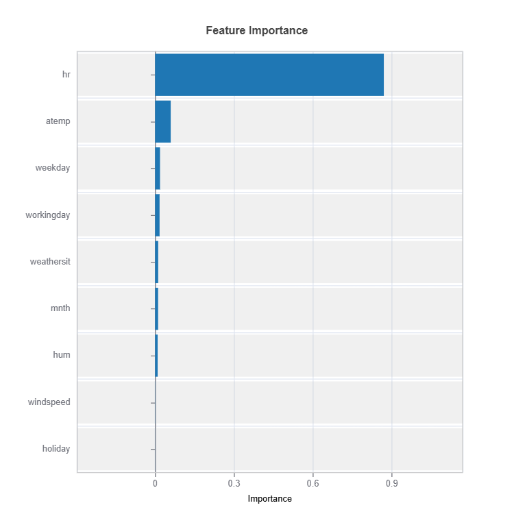
Feature Importance

Assess overall feature impact:

# Global feature importance
result = ts.interpret_fi()
# Plot the result
result.plot()

For the full list of arguments of the API see TestSuite.interpret_fi.

Importance Metrics:

• Based on variance of marginal effects

• Normalized to sum to 1

• Higher values indicate stronger influence

• Accounts for feature scale differences

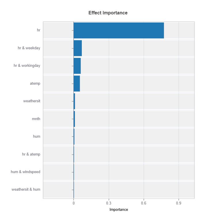
Effect Importance

Assess overall impact according to functional ANOVA components: main and interaction effect

# Global effect importance
result = ts.interpret_ei()
# Plot the result
result.plot()

For the full list of arguments of the API see TestSuite.interpret_ei.

Importance Metrics:

• Based on variance of individual functional ANOVA term effects (main or interaction effect)

• Higher values indicate stronger influence

Categorical Variables

• One-hot encoded automatically

• Can view importance per category

• Interpretable through reference levels

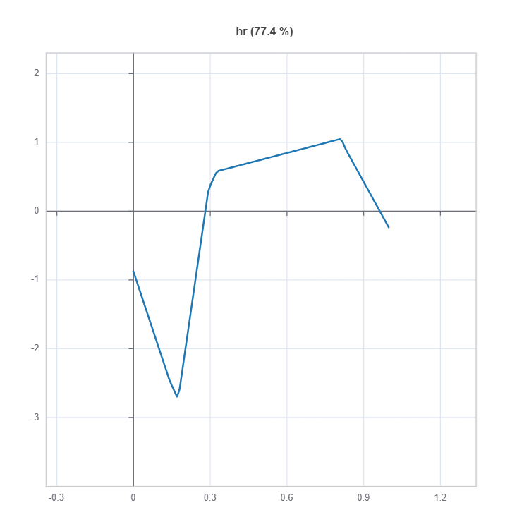
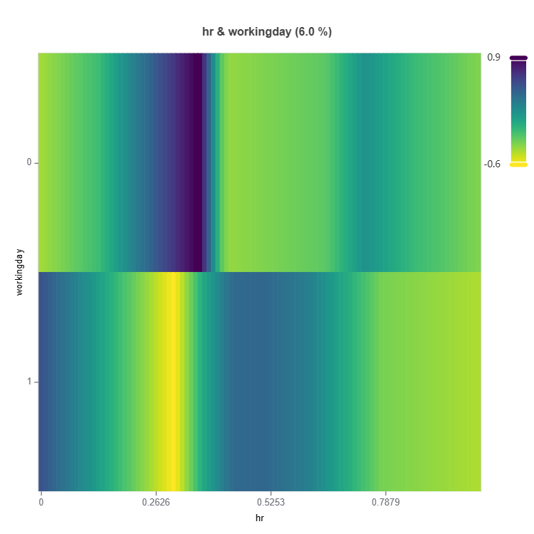
Global Effect Plot

Plot the main and interaction effect plot of features

# Main effect plot of feature: "hr"
result = ts.interpret_effects(features = "hr")
# Plot the result
result.plot()

# Interaction effect plot of features: "hr" and "weekday"
result = ts.interpret_effects(features = ("hr","workingday"))
# Plot the result
result.plot()

For the full list of arguments of the API see TestSuite.interpret_effects.

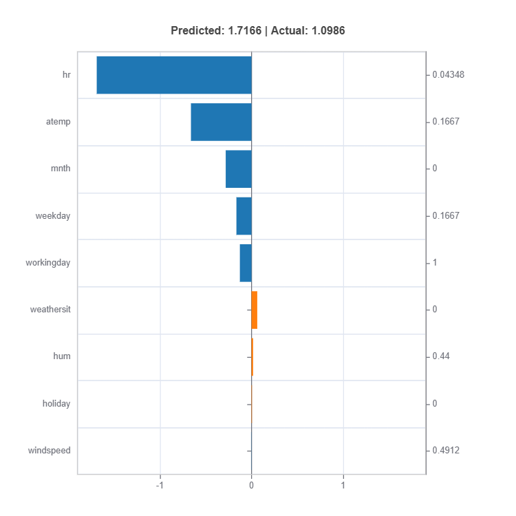
Local Interpretation

Individual Prediction Analysis

# Local interpretation for specific sample: sample_index = 10
result = ts.interpret_local_fi(sample_index = 10, centered = True)   # local feature importance
# Plot the result
result.plot()

result = ts.interpret_local_ei(sample_index = 10, centered = True)   # local effect importance
# Plot the result
result.plot()

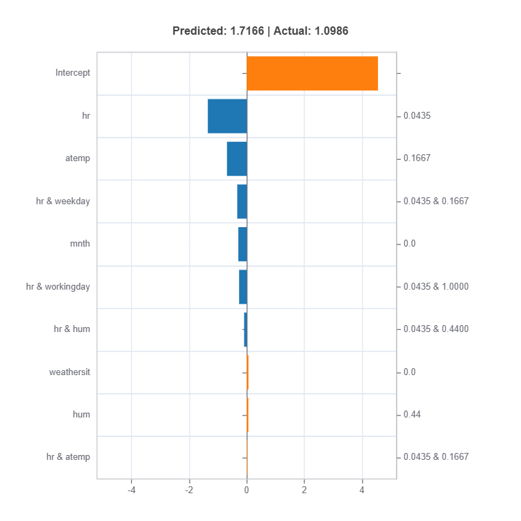
For the full list of arguments of the API see TestSuite.interpret_local_fi and TestSuite.interpret_local_ei .

Components:

• Feature or Effect contributions to prediction

• Feature or Effect values for the sample

• Comparison to average behavior

• Direction and magnitude of effects

Centering Options

1. Uncentered Analysis (centered=False):

   • Raw feature contributions

   • Direct interpretation

   • May have identifiability issues

2. Centered Analysis (centered=True):

   • Compares to population mean

   • More stable interpretation

   • Better for relative importance

Monotonicity Constraints in GAMI-Net

Enforcing monotonicity constraints to align with domain knowledge is often nneded to ensure model conceptual soundness. In many applications where GAMI-Net is deployed, certain input features should have a consistently positive or negative effect on predictions:

• In credit scoring, higher income should lead to better credit ratings

• In medical risk assessment, increased risk factors should result in higher risk scores

• In pricing models, larger product quantities should correspond to higher total costs

While GAMI-Net’s additive structure provides natural interpretability, explicitly enforcing monotonicity makes the model more reliable and trustworthy. Without monotonicity constraints, even interpretable models may learn relationships that violate logical domain constraints, particularly in regions with sparse training data.

Loss Function with Monotonicity Constraint in GAMI-Net

GAMI-Net augments its standard loss function with a monotonicity constraint penalty that operates on both main effects and interaction terms:

\[L_{total} = l(\theta) + \lambda \sum_{j \in S_1} \sum_{(j,k) \in S_2} \Omega(h_j, f_{jk}) + \gamma \sum_{i \in M} \mathbb{E}_x[\max(0, -\frac{\partial \hat{y}}{\partial x_i})^2]\]

where:

• \(l(\theta)\) is the base prediction loss

• \(\lambda \sum_{j \in S_1} \sum_{(j,k) \in S_2} \Omega(h_j, f_{jk})\) is the marginal clarity penalty

• \(\gamma\) is the monotonicity penalty coefficient

• \(M\) is the set of features that should be monotonic

• \(\frac{\partial \hat{y}}{\partial x_i}\) is the gradient of prediction with respect to feature i

Explanation

The loss function has three components working together to create an interpretable and conceptually sound model:

1. The prediction loss \(l(\theta)\) ensures accurate predictions.

2. The marginal clarity term \(\Omega(h_j, f_{jk})\) maintains clear separation between main effects and their interactions.

3. The monotonicity penalty \(\max(0, -\frac{\partial \hat{y}}{\partial x_i})^2\) enforces monotonic relationships for specified features by penalizing negative gradients.

This formulation is particularly powerful in GAMI-Net because it enforces monotonicity while preserving the model’s structured additive form. The monotonicity constraints apply to both individual feature effects and their interactions, ensuring that the entire model respects domain knowledge about feature relationships.

The strength of monotonicity enforcement can be tuned through \(\gamma\), allowing practitioners to balance between strict monotonicity and prediction accuracy. When \(\gamma\) is large, the model will strongly enforce monotonicity even if it means slightly reduced accuracy. When \(\gamma\) is smaller, the model has more flexibility to fit the data while still maintaining some monotonic tendency.

Implementation Considerations

When implementing monotonicity constraints in GAMI-Net:

• Provide the lists of input variables that have monotonically increasing and decreasing in the API: mono_increasing_list=(), mono_decreasing_list=()

• Start with a small monotonic regularization reg_mono and gradually increase it until desired monotonicity is achieved

• GAMI-Net is using sampling with sample size controlled by `mono_sample_size`to check monotonicity

• Evaluate both prediction performance and monotonicity violations

• Verify monotonicity holds for both main effects and interaction terms

• Consider using validation data to tune the reg_mono parameter

Examples

Example 1: Bike Sharing

The example below demonstrates how to use MoDeVa with its high-code APis for the Bike Sharing dataset from the UCI repository, which consists of 20,640 samples and 9 features, fetched by sklearn.datasets. The response variable MedHouseVal (Median Home Value) is continuous and is a regression problem.

• GAMINet Regression

Examples 2: Taiwan Credit

The second example below demonstrates how to use MoDeVa’s high-code APIs for the TaiwanCredit dataset from the UCI repository. This dataset comprises the credit card details of 30,000 clients in Taiwan from April 2005 to September 2005, and more information can be found on the TaiwanCreditData website. The FlagDefault variable serves as the response for this classification problem.

• GAMINet Classification

References

References

[Yang2020]

Zebin Yang, Aijun Zhang and Agus Sudjianto (2020). GAMI-Net: An Explainable Neural Network based on Generalized Additive Models with Structured Interactions, arXiv preprint arXiv:2003.07132.