Robustness

Robustness evaluates a model’s ability to perform reliably when exposed to input noise or changes, ensuring it remains accurate and stable under various conditions. In banking, robustness is essential to avoid issues like benign overfitting [Cui2023], which occurs when models fit noise in the training data but fail to generalize to new data. This section outlines key practices to test and enhance model robustness.

Noise sensitivity testing can be done by introducing small perturbations to input data and evaluate the impact on predictions. For instance, a slight change in a customer’s credit score or income level should not lead to a disproportionate shift in loan approval outcomes.

• Example: Add random noise to numeric features (e.g., credit score ±1%) and measure prediction stability.

• Goal: Ensure that predictions are not overly sensitive to minor data variations.

Investigating and Improving Model Robustness

MoDeVa provides a structured approach to investigate and enhance model robustness. The steps include:

1. Perturb Input Variables in Testing Data: Introduce controlled perturbations or noise to the input variables in the testing dataset. This simulates real-world scenarios where data may include slight variations, helping to evaluate the model’s sensitivity to changes.

2. Assess Performance Degradation: Evaluate how the introduced perturbations impact the model’s performance. Compare metrics such as accuracy, precision, recall, or mean squared error before and after perturbation to quantify the degradation.

3. Identify and Rank Sensitive Variables: Analyze the impact of perturbations on individual input variables. Rank the variables based on their sensitivity to noise, identifying those that contribute most to performance degradation.

4. Enhance Model Robustness: Implement improvements to address identified weaknesses, including:

   • Regularization Techniques: Apply L1/L2 penalties to reduce sensitivity to noise.

   • Feature Engineering: Refine or remove noisy variables to improve data quality.

   • Ensemble Methods: Use techniques like bagging or averaging to stabilize predictions.

   • Adversarial Training: Train the model with perturbed data to make it more robust to noise.

By systematically applying these steps, MoDeVa ensures models remain robust in the face of data variability and noise.

Input Perturbation for Robustness Test

To evaluate model robustness, MoDeVa supports two methods for perturbing input data:

Simple Perturbation with Normally Distributed Random Noise

This method adds random noise to input variables, drawn from a normal distribution, to simulate minor deviations in the data.

• Define fraction multipliers, \(k\) (e.g., 0.01, 0.02), to standard deviation (\(\sigma\)) for the noise.

• Generate random noise for each input feature:

  \[\text{perturbed value} = \text{original value} + k * \mathcal{N}(0, \sigma^2)\]

Use Case: Test sensitivity to small-scale, realistic random fluctuations in the data.

Quantile Perturbation with Uniform Noise

This method perturbs variables by adding uniform noise to their quantile space, preserving the data’s distribution.

• Convert input values into quantiles using the cumulative distribution function (CDF) of the variable:

  \[q = F(x)\]

  Where \(F(x)\) is the empirical CDF.

• Add uniform noise (\(\mathcal{U}(-\Delta, \Delta)\)) to the quantiles:

  \[q_{\text{perturbed}} = q + \mathcal{U}(-\Delta, \Delta)\]

  Choose \(\Delta\) based on the desired perturbation range in the quantile space.

• Map the perturbed quantiles back to the original data scale using the inverse CDF:

  \[x_{\text{perturbed}} = F^{-1}(q_{\text{perturbed}})\]

Use Case: Evaluate model robustness while preserving the original variable’s distributional characteristics.

Perturbation for Categorical Variable

For illustration, let’s assume we have three categories (A, B, and C). First of all, we summarize the frequency of each category in the data, e.g., 30%, 30%, and 40%, respectively. Then, each sample is perturbed with probability \(p\) (perturb_size) and kept unchanged with probability \(1-p\). For example, if \(p=0.3\), then 30% of the samples will be perturbed. If a sample is perturbed, it will be perturbed to A, B, and C with probability 30%, 30%, and 40%, respectively.

Practical Considerations

Choosing the Approach

• Simple Perturbation is straightforward and suitable for general robustness testing across all features.

• Quantile Perturbation is ideal for preserving the statistical properties of variables, especially for non-normal distributions or when dealing with features with specific value constraints (e.g., probabilities bounded between 0 and 1).

• Feature-specific design: choose perturbation techniques based on feature types (continuous vs. categorical)

• Perturbation magnitude: ensure perturbations reflect realistic scenarios.

Deciding the Maximum Perturbation Size To determine the maximum size of input perturbations for robustness testing, a linear model can be used as a benchmark. The maximum perturbation size is defined as the point where the model’s performance drops to a level below that of the linear model.

1. Train a Linear Model Benchmark: train a simple linear model using the same dataset to serve as a baseline for comparison.

2. Incrementally Apply Perturbations: apply increasing levels of perturbations to the input data using the chosen perturbation method (e.g., normal noise or quantile noise).

3. Monitor Model Performance: evaluate the performance of the model at each perturbation level, tracking metrics such as accuracy, precision, recall, or mean squared error.

4. Identify the Maximum Perturbation Bound: determine the largest perturbation size where the model’s performance remains above that of the linear benchmark. This size is used as the maximum allowable perturbation.

By applying these perturbation techniques, MoDeVa allows a thorough assessment of model robustness against both realistic and structured input variability.

Robustness Analysis in MoDeVa

Data Setup

from modeva import DataSet
## Create dataset object holder
ds = DataSet()
## Loading MoDeVa pre-loaded dataset "Bikesharing"
ds.load(name="BikeSharing")
## Preprocess the data
ds.scale_numerical(features=("cnt",), method="log1p") # Log transfomed target
ds.set_feature_type(feature="hr", feature_type="categorical") # set to categorical feature
ds.set_feature_type(feature="mnth", feature_type="categorical")
ds.scale_numerical(features=ds.feature_names_numerical, method="standardize") # standardized numerical features
ds.set_inactive_features(features=("yr", "season", "temp")) # deactivate some features
ds.preprocess()
## Split data into training and testing sets randomly
ds.set_random_split()

Model Setup

# Regression tasks using lightGBM and xgboost
from modeva.models import MoLGBMRegressor, MoXGBRegressor

# for lightGBM
model_lgbm = MoLGBMRegressor(name = "LGBM_model", max_depth=2, n_estimators=100)
# for xgboost
model_xgb = MoXGBRegressor(name = "XGB_model", max_depth=2, n_estimators=100)
# for catboost

Model Training

# train model with input: ds.train_x and target: ds.train_y
model_lgbm.fit(ds.train_x, ds.train_y)
model_xgb.fit(ds.train_x, ds.train_y)

Reporting and Diagnostic Setup

# Create a testsuite that bundles dataset and model
from modeva import TestSuite
ts = TestSuite(ds, model_lgbm) # store bundle of dataset and model in fs

Robustness Assessment

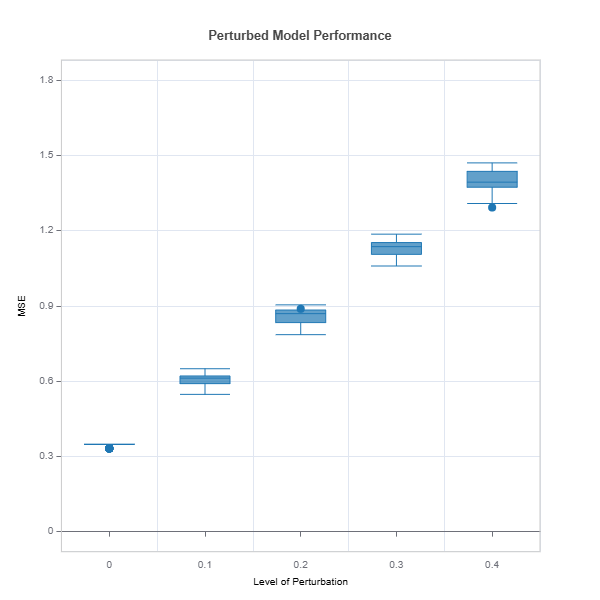
Performance degradation is evaluated by comparing the selected performance metrics under a set noise perturbation sizes.

# robustness analysis
ts = TestSuite(ds, model_lgbm)
   results = ts.diagnose_robustness(
   perturb_features=None,
   noise_levels=(0.1, 0.2, 0.3, 0.4),
   metric="MSE")
results.plot()

For the full list of arguments of the API see TestSuite.diagnose_robustness.

Identification of Robustness Issue and Impactful Variables

• Apply slicing technique to identify variables and their intervals with the most performance degradation

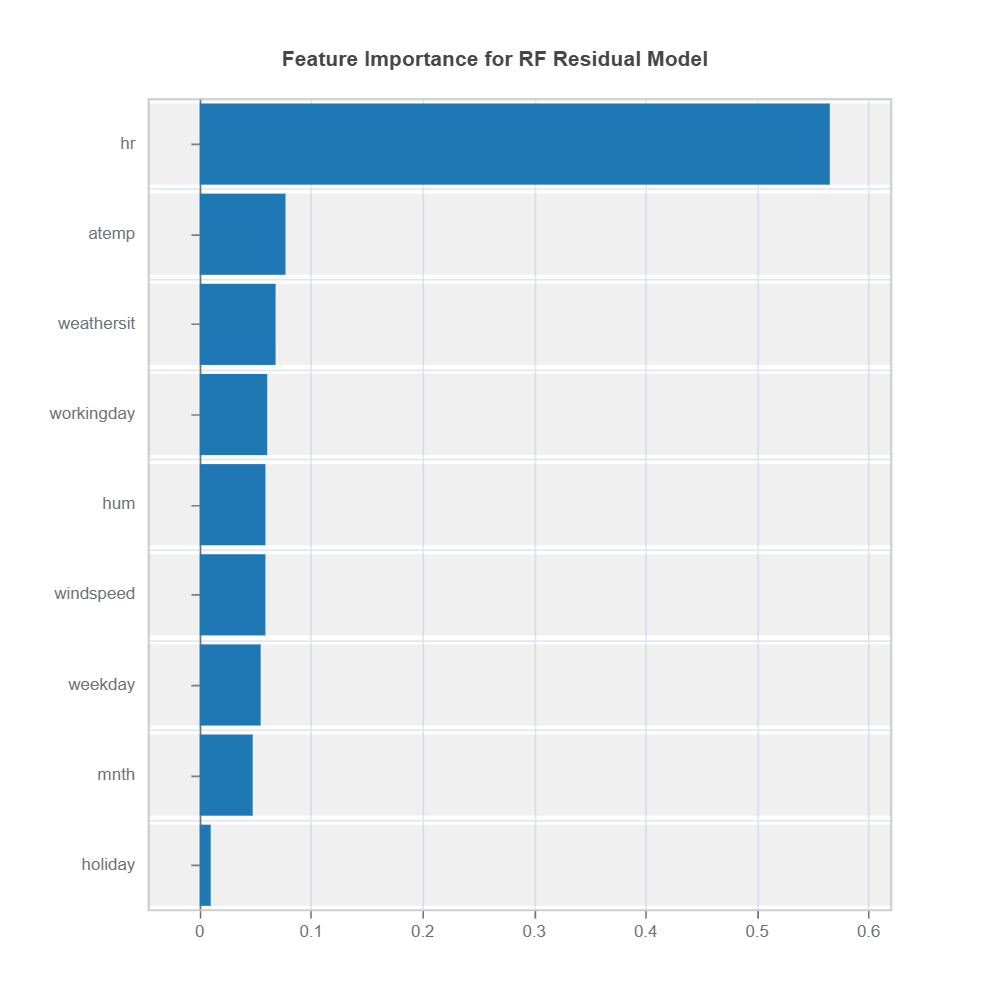
• Fit inherently interpretable model (e.g., xgboost depth-2) with error degradation as target and plot the effects (main or interaction) as well as variable importance with respected to robustness measure.

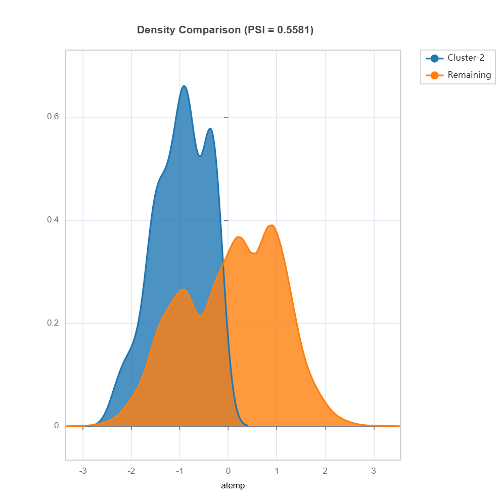
• Select sub-samples with less robust and visualize and compare the distributions between less robust vs. the rest. Distribution difference can be quantified using measure such as PSI.

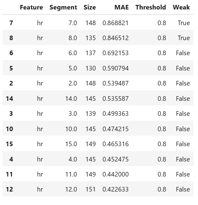
Univariate robustness slicing

Below is an example of slicing on

• features=”hr”

• perturbaion on perturb_features=(“hum”, “atemp”)

• perturbation size noise_levels=0.1

• binning method is automatically determined by xgboost depth-1, method=”auto-xgb1”

• threshold = 0.8 is the weak region threshold

results = ts.diagnose_slicing_robustness(
   features="hr",
   perturb_features=("hum", "atemp"),
   noise_levels=0.1,
   metric="MAE",
   method="auto-xgb1",
   threshold=0.8
results.table

For the full list of arguments of the API see TestSuite.diagnose_slicing_robustness.

Distribution difference for a specific feature

# import get_data_info from TestSuite utility
from modeva.testsuite.utils.slicing_utils import get_data_info
# retrieve result for "hr" feature
data_info = get_data_info(res_value=results.value)["hr"]
# apply drift test to rank distributional difference
data_results = ds.data_drift_test(
   **data_info,
   distance_metric="PSI",
   psi_method="uniform",
   psi_bins=10)
data_results.plot("summary")

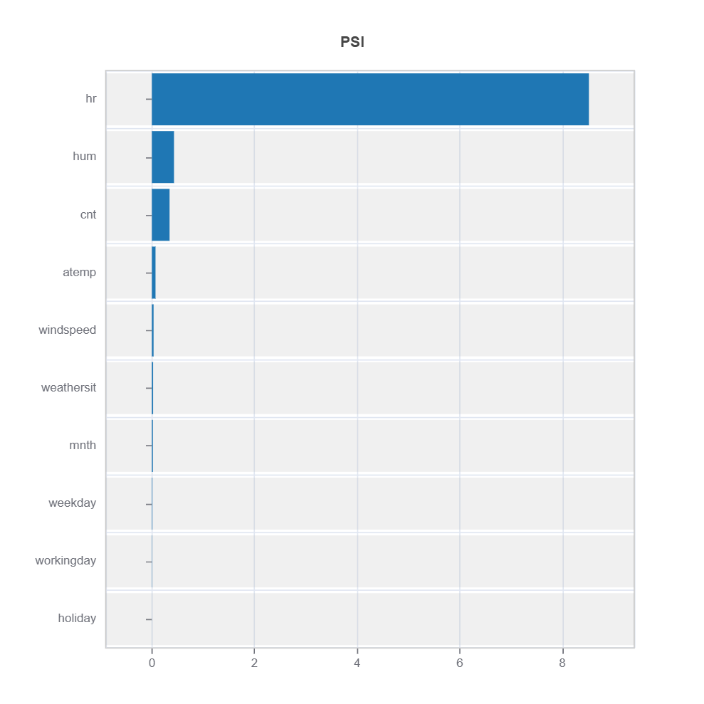
The results of distribution difference from TestSuite.diagnose_slicing_robustness is evaluated using DataSet.data_drift_test

• Percent of worst sample = 0.1 (10%) is selected for distribution shift

• Metrics: PSI with 10 uniform binning is used for calculation.

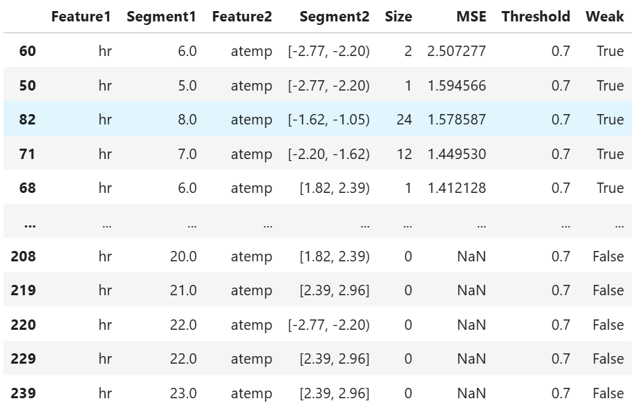
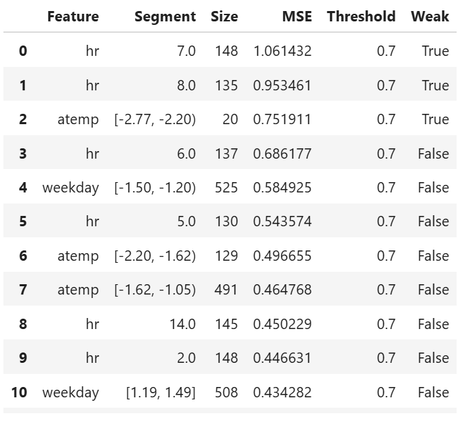
Bivariate Slicing

Example of bivariate slicing on features=(“hr”, “atemp”)

results = ts.diagnose_slicing_robustness(
   features=("hr", "atemp"),
   perturb_features=("hum", "atemp"),
   noise_levels=0.1,
   metric="MSE",
   threshold=0.7)
results.table

Multiple Univariate Slicing

results = ts.diagnose_slicing_robustness(
   features=(("hr",), ("atemp",), ("weekday",)),
   perturb_features=("atemp", "hum"),
   noise_levels=0.1,
   perturb_method="quantile",
   metric="MSE",
   threshold=400)
results.table

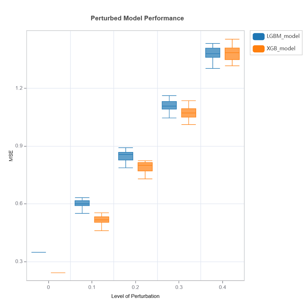
Robustness Comparison

Robustness of several models can be compared as follows:

tsc = TestSuite(ds, models=[model_lgbm, model_xgb])
# robustness comparison of 2 models specified in tsc
results = tsc.compare_robustness(
   perturb_features=("hr", "atemp"),
   noise_levels=(0.1, 0.2, 0.3, 0.4),
   perturb_method="quantile",
   metric="MSE")
results.plot()

Check the API reference for detail arguments of TestSuite.compare_robustness.

The robustness of multiple models can be compared for each feature using variable slicing:

results = tsc.compare_slicing_robustness(
   features="hr",
   noise_levels=0.1,
   method="quantile",
   metric="MSE")
results.plot()

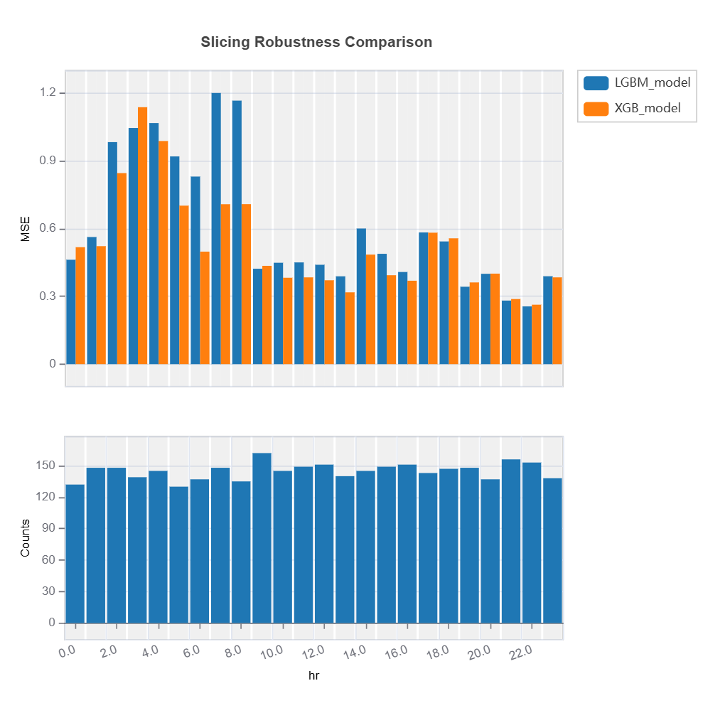
Check the API reference for detail arguments of TestSuite.compare_slicing_robustness.

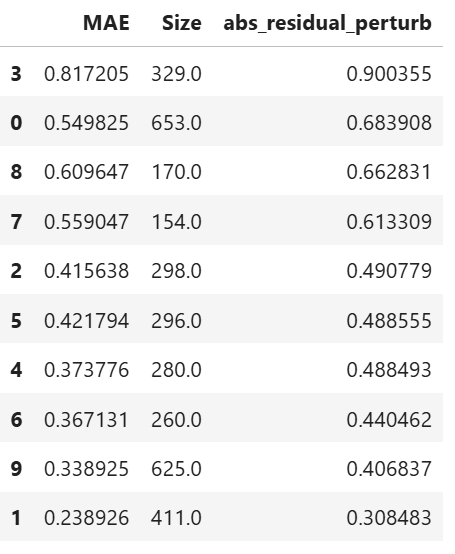
Supervised Machine Learning: Random Forest Clustering

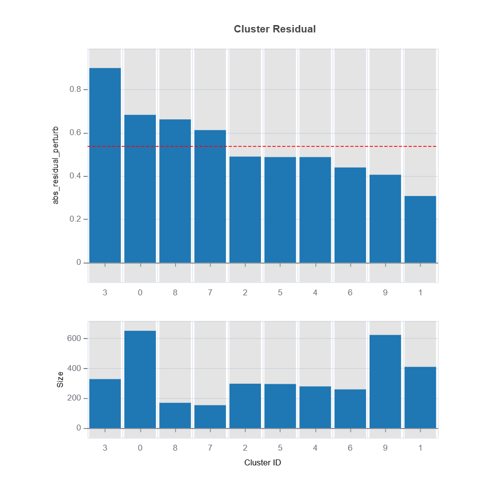
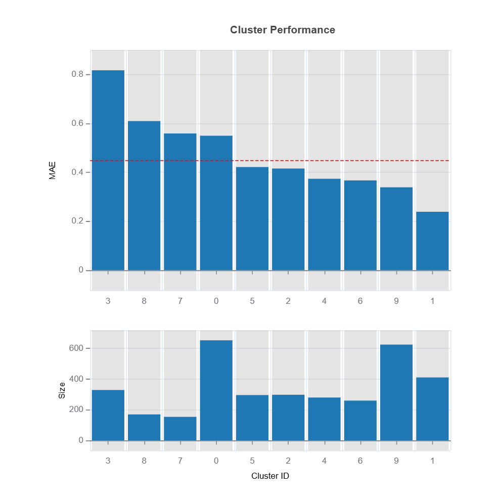
Change of residuals due to perturbation of features can be used as a target clustering variable for supervised machine learning clustering using Random Forest proximity..

results = ts.diagnose_residual_cluster(
   dataset="test", # dataset
   response_type="abs_residual_perturb", # response type for robustness clustering
   metric="MAE", # metric
   n_clusters=10, # number of clusters
   cluster_method="pam", # clustering method
   sample_size=2000, # sample size
   rf_n_estimators=100, # number of trees
   rf_max_depth=5, # max depth of trees
)
 results.table #
 results.plot() #

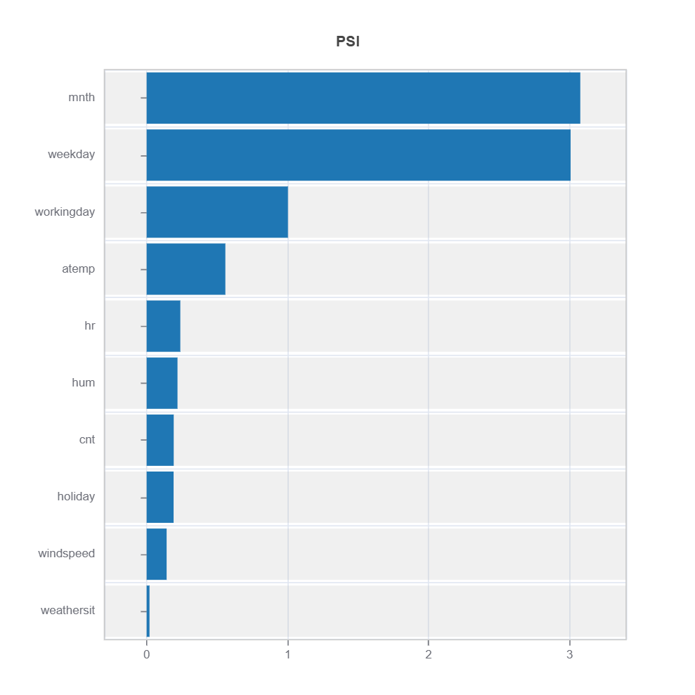
The following code shows how to identify the high-uncertainty region and interpret the results:

cluster_id = 2 # cluster id
data_results = ds.data_drift_test(
   **results.value["clusters"][cluster_id]["data_info"], # use the cluster_id
   distance_metric="PSI", # distance metric using PSI
   psi_method="uniform", # psi method using uniform distribution
   psi_bins=10 # psi bins
)
data_results.plot("summary") # plot summary of data drift test
data_results.plot(name=('density', 'mnth')) # plot density plot for feature "mnth"

Strategies for Addressing Model Weaknesses

Data-Centric Approaches

1. Feature Engineering:

Based on weakness patterns (features causing robustness issue): * Perform feature transformation for those causing robustness issues

Model-Centric Approaches

1. Architecture Modifications:

Based on the robsutness patterns:

• Choose modeling alternative that is more robust (e.g., controlling tree depth in GBDT. number of nodes in neural networks, choosing basis functions in gradient boosted tree: constant or linear (LinearTree) at the terminal nodes)

• Incorporate domain knowledge via constraints (e.g., monotonicity)

2. Loss Function Adjustments:

• Apply regularization to reduce overfitting

L1 Regularization (Lasso):

\[L_{\text{total}} = L_{\text{pred}} + \lambda_1 \sum_{i} |w_i|\]

Sparsity promotes robustness.

L2 Regularization (Ridge):

\[L_{\text{total}} = L_{\text{pred}} + \lambda_2 \sum_{i} w_i^2\]

Equivalently injecting noise to training data has similar effect as L2 regularization.

Local Regularization

\[L_{new}(X,y) = L_{original}(X,y) + \lambda W(X)R(X)\]

where:

• \(R(X)\) is an indicator for weak regions

• \(\lambda\) balances overall performance vs local improvement by applying stronger regularization or adversarial (perturbed) training samples

Early stopping in the training phase This applicable to both gradient boosted decision tree and neural networks.

Examples

Example 1: Bike Sharing

The example below demonstrates how to use MoDeVa with its high-code APis for the Bike Sharing dataset from the UCI repository, which consists of 20,640 samples and 9 features, fetched by sklearn.datasets. The response variable MedHouseVal (Median Home Value) is continuous and is a regression problem.

• Robustness Analysis (Regression)

Examples 2: Taiwan Credit

The second example below demonstrates how to use MoDeVa’s high-code APIs for the TaiwanCredit dataset from the UCI repository. This dataset comprises the credit card details of 30,000 clients in Taiwan from April 2005 to September 2005, and more information can be found on the TaiwanCreditData website. The FlagDefault variable serves as the response for this classification problem.

• Robustness Analysis (Classification)

References

[Cui2023]

Shijie Cui, Agus Sudjianto, Aijun Zhang and Runze Li (2023). Enhancing Robustness of Gradient-Boosted Decision Trees through One-Hot Encoding and Regularization, arXiv preprint arXiv:2304.13761.