Resilience

Resilience is the ability of a model to maintain accurate performance despite changes in input data distribution or external factors. In banking, this is particularly important due to shifting economic conditions, evolving customer behaviors, and changing regulatory environments—all of which can affect model performance over time. For instance, variations in input data such as income levels, employment rates, or customer behavior can lead to reduced predictive accuracy.

To evaluate a model’s resilience, one effective approach is to assess its performance across different behavioral segments or clusters. If significant discrepancies in performance are observed across these segments, it may indicate the need for further analysis or the development of segment-specific models to address these variations.

Investigating and Improving Model Resilience in MoDeVa

In MoDeVa, investigating and improving model resilience involves the following steps:

1. Apply Distribution Shift Scenarios: Analyze the circumstances and distribution shift conditions under which the model’s performance declines to understand potential vulnerabilities.

2. Assess Variability and Segment Performance: Evaluate the model’s performance across different segments or clusters to identify areas of inconsistency or significant variability.

3. Determine Impactful Variables: Identify key variables whose distributional shifts have the greatest impact on performance degradation, helping to prioritize areas for improvement.

4. Enhance the Model: Address the identified issues by refining the model, such as through further analysis, introducing segment-specific models, or other tailored adjustments.

Distribution Shift Scenarios

There are many scenarios that can be employed to simulate a shift between the training/testing (or overall) distribution and the deployment distribution, MoDeVa provides the following scenarios:

1. Drift to Worst Performing Samples Idea: Identify samples on which the model’s performance is poorest measured by error metrics or mispredictions—and simulate drift by increasing their proportion. Rationale: This can mimic a “worst-case” scenario where the deployment data disproportionately resembles the “hard” cases, revealing vulnerabilities in the model.

2. Drift to Clusters (KMeans) to the Worst Performing Cluster Idea: Use a clustering algorithm (e.g., k-means) on the feature space to segment the data. Then, determine which cluster exhibits the worst performance and simulate drift by focusing on this subgroup. Rationale: Clustering can capture latent subpopulations in the data. If one cluster consistently underperforms, it may represent a niche or anomalous group, and simulating drift toward this cluster can expose model weaknesses specific to that segment.

3. Drift to the Edge (Outer Side of the Distribution) Idea: Identify samples that lie at the periphery of the overall data distribution. This involves using distance metrics (Mahalanobis distance) to quantify how “far” a sample is from the center of the data. Rationale: Edge cases are typically less represented during training and can behave like out-of-distribution (OOD) samples. Shifting towards these samples can test the model’s ability to generalize to more extreme, less typical cases.

4. Drift to Distribution of Samples that are Hardest to Predict Idea: Determine which samples the model finds most uncertain or difficult to predict—-high predictive entropy, low confidence scores, or high error rates. Rationale: These samples are where the model is least reliable. By simulating a scenario where these “hard” samples become more common, you can assess how well the model handles uncertainty and whether strategies like uncertainty-aware training or selective prediction might help.

Perormance Degradation Assessment

• Performance Metrics: In each case, we track performance metrics (e.g., accuracy, F1 score, MSE) under the drifted distribution to quantify degradation.

• Robustness & Adaptation: These experiments can inform how to improve model robustness—whether through reweighting, data augmentation, adversarial training, or domain adaptation techniques.

• Simulation Strategy: The shift is simulated gradually (e.g., by progressively increasing the proportion of “drifted” samples) to observe the degradation curve.

By comparing the model’s performance across these different drift scenarios, you gain valuable insights into which aspects of the data the model struggles with and how it might perform in more challenging real-world conditions.

Resilience Analysis in MoDeVa

Performance degradation is evaluated by comparing the selected performance metrics under specific distribution shift scenarios to a baseline established from the full training or testing data distribution. The distribution shift is represented as a subset of the baseline data, tailored to the chosen scenario. This allows for a targeted analysis of how the model performs under different conditions and highlights areas where resilience improvements may be needed.

Data Setup

from modeva import DataSet
## Create dataset object holder
ds = DataSet()
## Loading MoDeVa pre-loaded dataset "Bikesharing"
ds.load(name="BikeSharing")
## Preprocess the data
ds.scale_numerical(features=("cnt",), method="log1p") # Log transfomed target
ds.set_feature_type(feature="hr", feature_type="categorical") # set to categorical feature
ds.set_feature_type(feature="mnth", feature_type="categorical")
ds.scale_numerical(features=ds.feature_names_numerical, method="standardize") # standardized numerical features
ds.set_inactive_features(features=("yr", "season", "temp")) # deactivate some features
ds.preprocess()
## Split data into training and testing sets randomly
ds.set_random_split()

Model Setup

# Regression tasks using lightGBM and xgboost
from modeva.models import MoLGBMRegressor, MoXGBRegressor

# for lightGBM
model_lgbm = MoLGBMRegressor(name = "LGBM_model", max_depth=2, n_estimators=100)
# for xgboost
model_xgb = MoXGBRegressor(name = "XGB_model", max_depth=2, n_estimators=100)
# for catboost

Model Training

# train model with input: ds.train_x and target: ds.train_y
model_lgbm.fit(ds.train_x, ds.train_y)
model_xgb.fit(ds.train_x, ds.train_y)

Reporting and Diagnostic Setup

# Create a testsuite that bundles dataset and model
from modeva import TestSuite
ts = TestSuite(dataset, model_lgbm) # store bundle of dataset and model in fs

Resilience Assessment

# resilience assessment using Worst-Sample scenario
results = ts.diagnose_resilience(method="worst-sample", metric="MSE")
results.plot()

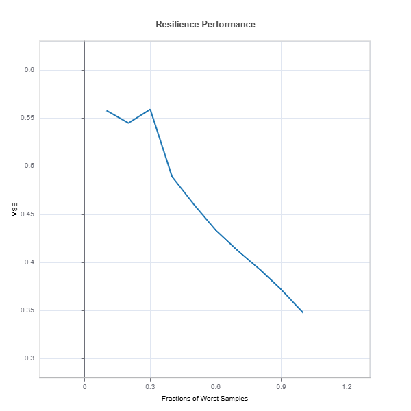
# resilience assessment using Worst-Cluster scenario with maximum number of custers 'n_clusters=5'
results = ts.diagnose_resilience(method="worst-cluster", n_clusters=5, metric="MSE")
results.plot()

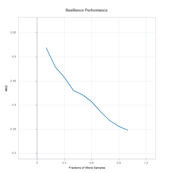
# resilience assessment using edge (outer) sample scenario
results = ts.diagnose_resilience(method="outer-sample", metric="MSE")
results.plot()

# resilience assessment using hard sample to predict scenario
results = ts.diagnose_resilience(method="hard-sample", metric="MSE")
results.plot()

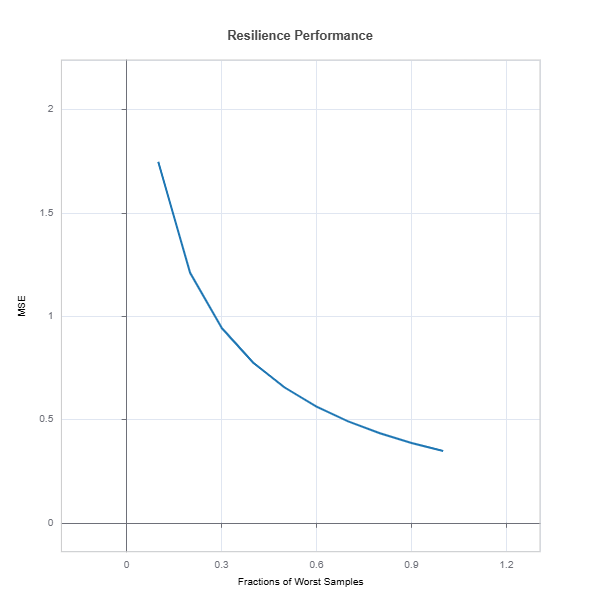
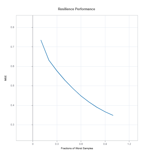
The results.plot() shows performance degradation due to distribution shift

For the full list of arguments of the API see TestSuite.diagnose_resilience.

Measuring Distribution Drift

Univariate distribution shifts are evaluated using the following metrics:

• Jensen-Shannon Divergence (Population Stability Index): Measures the similarity between two probability distributions, identifying variable distribution shifts.

• Wasserstein Distance: Quantifies the cost of transforming one distribution into another, offering insights into the extent of the shift.

• Kolmogorov-Smirnov (KS) Statistic: Identifies the maximum difference between the cumulative distributions of two samples, pinpointing significant deviations.

To assess the direction of distribution shifts and determine variable importance, these metrics are used to rank variables. This ranking highlights the variables most affected by distribution changes, helping prioritize them for further investigation and potential remediation to mitigate performance degradation. This section presents both theoretical (continuous) and computational (discrete) formulations of key distribution shift metrics.

Jensen-Shannon Divergence

Continuous Formulation:

For probability density functions of shifted distribution p(x) and reference distribution q(x):

\[JSD(P||Q) = \frac{1}{2}\int p(x)\log\frac{p(x)}{m(x)}dx + \frac{1}{2}\int q(x)\log\frac{q(x)}{m(x)}dx\]

where:

• \(m(x) = \frac{1}{2}(p(x) + q(x))\)

Discrete Formulation (PSI):

For binned data with K bins:

\[PSI = \sum_{i=1}^K (p_i - q_i)\log\frac{p_i}{q_i}\]

where:

• \(p_i\) and \(q_i\) are proportions of observations in bin i

• Small constant ε (e.g., 1e-6) is added to avoid log(0)

• \(p_i = \frac{n_i + \epsilon}{\sum_j (n_j + \epsilon)}\)

Wasserstein Distance

Continuous Formulation:

For cumulative distribution functions F(x) and G(x):

\[W(P,Q) = \int_{-\infty}^{\infty} |F(x) - G(x)|dx\]

Discrete Formulation:

For empirical distributions with sorted values \(\{x_i\}_{i=1}^n\) and \(\{y_i\}_{i=1}^n\):

\[W(P,Q) = \sum_{i=1}^n |F_n(x_i) - G_n(x_i)|\Delta x_i\]

where:

• \(F_n\) and \(G_n\) are empirical CDFs

• \(\Delta x_i\) is the difference between consecutive sorted unique values

• For equal-sized samples: \(F_n(x_i) = \frac{rank(x_i)}{n}\)

Kolmogorov-Smirnov Statistic

Continuous Formulation:

\[KS = \sup_{x \in \mathbb{R}} |F(x) - G(x)|\]

Discrete Formulation:

For empirical distributions:

\[KS = \max_{i} |F_n(x_i) - G_n(x_i)|\]

where:

• \(x_i\) are the sorted unique values from combined samples

• \(F_n\) and \(G_n\) are empirical CDFs

Feature Drift Impacts

# resilience assessment using Worst-Sample scenario
data_results = ds.data_drift_test(
   **results.value[0.1]["data_info"],
   distance_metric="PSI",
   psi_method="uniform",
   psi_bins=10)
data_results.plot()

The results of distributional drift from TestSuite.diagnose_resilience is evaluated using DataSet.data_drift_test

• Percent of worst sample = 0.1 (10%) is selected for distribution shift

• Metrics: PSI with 10 uniform binning is used for calculation.

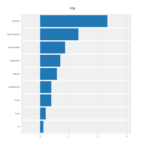
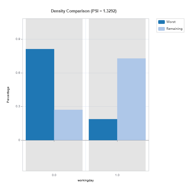
data_results.plot() displays the following results:

• Summary of distribution shift for all the features ranked by PSI

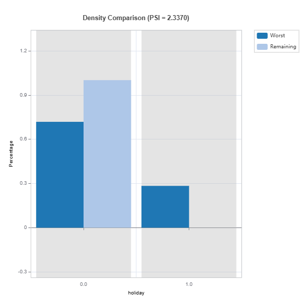
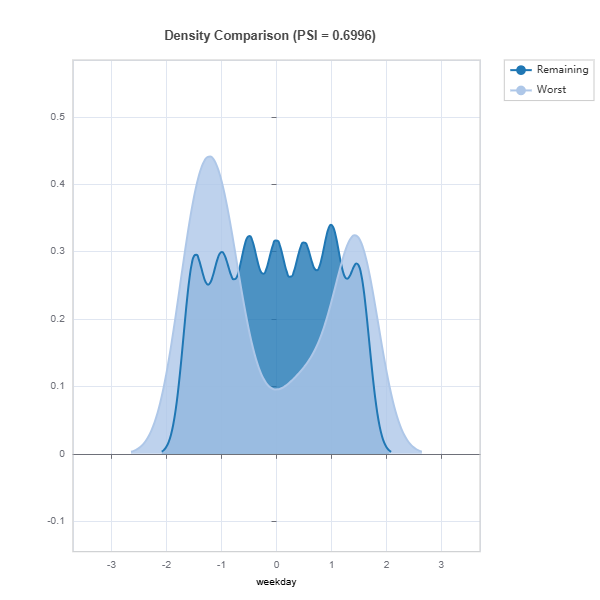
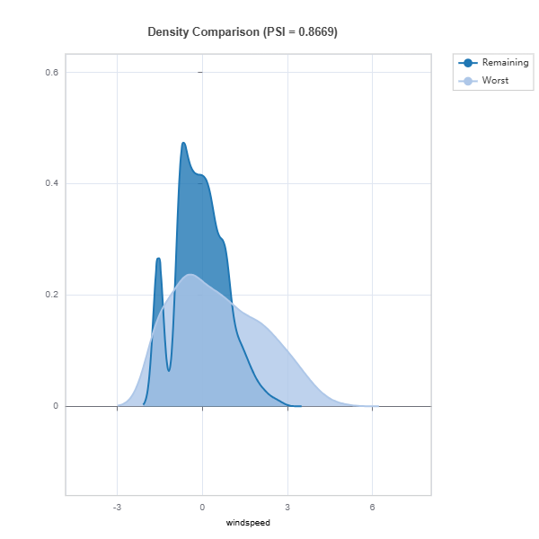
• Marginal density comparison of distribution shift

• Marginal histogram comparison of distribution shift

the univariate distribution shifts and the summary of features ranked according to their PSIs.

Resilience Comparison

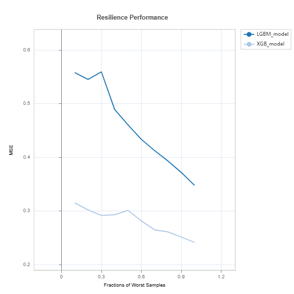
Resilience of several models can be compared as follows:

tsc = TestSuite(ds, models=[model_lgbm, model_xgb])
# resilience assessment using Worst-Cluster scenario
results = tsc.compare_resilience(n_clusters=5, method="worst-cluster", metric="MSE")
results.plot()

Check the API reference for detail arguments of TestSuite.compare_resilience.

Strategies for Addressing Model Weaknesses

Data-Centric Approaches

1. Targeted Data Augmentation:

For regions with poor performance:

\[R_{weak} = \{X: W(X) > Q_{1-β}(W) \text{ or } V(X,y) = 1\}\]

Solutions:

• Collect additional samples in \(R_{\text{weak}}\)

• Active learning in weak regions

2. Feature Engineering:

Based on weakness patterns:

• Create interaction terms for regions with nonlinear patterns

• Develop domain-specific features where performance is poor

• Improve feature engineering where performance is poor

Model-Centric Approaches

1. Local Model Enhancement:

For identified weak regions \(R_{\text{weak}}\):

\[\begin{split}f_{enhanced}(X) = \begin{cases} f_{local}(X) & \text{if } X \in R_{weak} \\ f_{global}(X) & \text{otherwise} \end{cases}\end{split}\]

Strategies:

• Train specialized models for \(R_{\text{weak}}\) (segmentation)

• Ensemble models with region-specific weights (Mixture of Experts)

2. Architecture Modifications:

Based on weakness patterns:

• Incorporate domain knowledge via constraints

• Use mixture of experts to reduce performance heterogeneity

3. Loss Function Adjustments:

\[L_{new}(X,y) = L_{original}(X,y) + \lambda W(X)R(X)\]

where:

• \(R(X)\) is an indicator for weak regions

• \(\lambda\) balances overall performance vs local improvement

Examples

Example 1: Bike Sharing

The example below demonstrates how to use MoDeVa with its high-code APis for the Bike Sharing dataset from the UCI repository, which consists of 20,640 samples and 9 features, fetched by sklearn.datasets. The response variable MedHouseVal (Median Home Value) is continuous and is a regression problem.

• Resilience Analysis (Regression)

Examples 2: Taiwan Credit

The second example below demonstrates how to use MoDeVa’s high-code APIs for the TaiwanCredit dataset from the UCI repository. This dataset comprises the credit card details of 30,000 clients in Taiwan from April 2005 to September 2005, and more information can be found on the TaiwanCreditData website. The FlagDefault variable serves as the response for this classification problem.

• Resilience Analysis (Classification)