Performance and Residual Analysis#

Measuring the performance of a machine learning model is critical for understanding its accuracy, reliability, and suitability for real-world applications. Proper evaluation ensures that the model meets its intended objectives, generalizes well to unseen data, and operates effectively under practical conditions.

Introduction#

Why Measure Model Performance?

Accuracy Assessment: - Quantify how well the model predicts outcomes for unseen data.
Comparison of Models: - Select the best-performing model among multiple candidates.
Bias and Variance Analysis: - Detect overfitting (high variance) or underfitting (high bias).
Business Impact: - Translate performance metrics into actionable insights, such as improved decision-making or cost reduction.

Key Concepts in Model Performance Measurement

Evaluation Metrics: - Metrics depend on the type of task:
- Classification: Accuracy, precision, recall, F1-score, AUC-ROC.
- Regression: Mean squared error (MSE), mean absolute error (MAE), R-squared.
Data Splitting: - Split the dataset into training, validation, and testing subsets for reliable evaluation.
Cross-Validation: - Use k-fold cross-validation to estimate performance across multiple data splits.
Real-World Validation: - Test the model with data that simulates real-world scenarios, such as temporal validation or external datasets.

Classification Metrics#

Accuracy:

$Accuracy = \frac{TP + TN}{TP + TN + FP + FN}$

Measures the proportion of correctly classified samples.

Precision:

$Precision = \frac{TP}{TP + FP}$

Evaluates the proportion of true positives among predicted positives.

Recall (Sensitivity):

$Recall = \frac{TP}{TP + FN}$

Measures the proportion of true positives among all actual positives.

F1-Score:

$F1-Score = 2 \cdot \frac{Precision \cdot Recall}{Precision + Recall}$

Harmonic mean of precision and recall.

Area Under the Curve (AUC-ROC):

$AUC-ROC = \int_{0}^{1} T P R (F P R^{- 1} (x)) d x$

Measures the ability of the model to distinguish between classes, plotting the True Positive Rate (TPR) against the False Positive Rate (FPR) across thresholds. A value of 1.0 represents perfect classification.

Log Loss (Cross-Entropy Loss):

$Log Loss = - \frac{1}{n} \sum_{i = 1}^{n} [y_{i} \log (p_{i}) + (1 - y_{i}) \log (1 - p_{i})]$

Where: - $y_{i}$ : True label (1 for positive, 0 for negative). - $p_{i}$ : Predicted probability for the positive class.

Log Loss penalizes predictions that are confident but incorrect. Lower values indicate better performance.

Brier Score

$Brier Score = \frac{1}{n} \sum_{i = 1}^{n} (p_{i} - y_{i})^{2}$

Evaluates the accuracy of predicted probabilities, where $p_{i}$ is the predicted probability for the positive class, and $y_{i}$ is the true label (1 for positive, 0 for negative). Lower values indicate better performance.

Regression Metrics#

Mean Squared Error (MSE):

$MSE = \frac{1}{n} \sum_{i = 1}^{n} ({\hat{y}}_{i} - y_{i})^{2}$

Average squared difference between predictions ( $\hat{y}$ ) and actual values ( $y$ ).

Mean Absolute Error (MAE):

$MAE = \frac{1}{n} \sum_{i = 1}^{n} | {\hat{y}}_{i} - y_{i} |$

Average absolute difference between predictions and actual values.

R-Squared (Coefficient of Determination):

$R^{2} = 1 - \frac{\sum_{i = 1}^{n} ({\hat{y}}_{i} - y_{i})^{2}}{\sum_{i = 1}^{n} (y_{i} - \bar{y})^{2}}$

Proportion of variance in the target variable explained by the model.

Mean Average Precision (MAP):

$MAP = \frac{1}{Q} \sum_{q = 1}^{Q} \frac{1}{m} \sum_{k = 1}^{m} P (k)$

Averages precision at each rank position for all queries.

Challenges in Measuring Model Performance#

Data Imbalance: - Metrics like accuracy may be misleading for imbalanced datasets; consider using precision, recall, or F1-score.
Overfitting/Underfitting: - Overfitting occurs when the model performs well on training data but poorly on unseen data. Underfitting results from insufficient learning of patterns in the data.
Real-World Applicability: - The model’s performance in lab conditions may not generalize to real-world scenarios.

Performance Evaluation in MoDeVa#

Data Setup

from modeva import DataSet
## Create dataset object holder
ds = DataSet()
## Loading MoDeVa pre-loaded dataset "Bikesharing"
ds.load(name="BikeSharing")
## Preprocess the data
ds.scale_numerical(features=("cnt",), method="log1p") # Log transfomed target
ds.set_feature_type(feature="hr", feature_type="categorical") # set to categorical feature
ds.set_feature_type(feature="mnth", feature_type="categorical")
ds.scale_numerical(features=ds.feature_names_numerical, method="standardize") # standardized numerical features
ds.set_inactive_features(features=("yr", "season", "temp")) # deactivate some features
ds.preprocess()
## Split data into training and testing sets randomly
ds.set_random_split()

Model Setup

# Regression tasks using lightGBM and xgboost
from modeva.models import MoLGBMRegressor, MoXGBRegressor

# for lightGBM
model_lgbm = MoLGBMRegressor(name = "LGBM_model", max_depth=2, n_estimators=100)
# for xgboost
model_xgb = MoXGBRegressor(name = "XGB_model", max_depth=2, n_estimators=100)
# for catboost

Model Training

# train model with input: ds.train_x and target: ds.train_y
model_lgbm.fit(ds.train_x, ds.train_y)
model_xgb.fit(ds.train_x, ds.train_y)

Reporting and Diagnostic Setup

# Create a testsuite that bundles dataset and model
from modeva import TestSuite
ts = TestSuite(ds, model_lgbm) # store bundle of dataset and model in fs
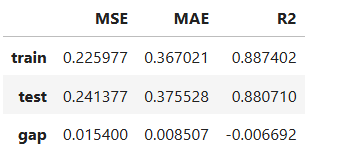
# Evaluate performance and summarize into table
results = ts.diagnose_accuracy_table(train_dataset="train", test_dataset="test",
                                  metric=("MAE", "MSE", "R2"))
results.table

For the full list of arguments of the API see TestSuite.diagnose_accuracy_table.

Residual Analysis#

Residual analysis is a diagnostic tool used in machine learning and statistics to evaluate the performance of a model by analyzing the differences between actual and predicted values. These differences, known as residuals, provide insights into how well the model fits the data and where it might struggle.

The residual for a given observation is calculated as:

Residual = Actual Value - Predicted Value

For regression problems, the residual measures the error in the model’s prediction for each data point. For classification problems, residuals are typically expressed as misclassification errors or the difference between predicted probabilities and true labels.

Purpose of Residual Analysis#

Model Fit: - Identify whether the model captures the underlying patterns in the data or if there are systematic errors.
Error Distribution: - Check whether residuals are randomly distributed, which indicates a well-fitting model. Systematic patterns in residuals suggest that the model is underperforming or mis-specified.
Outlier Detection: - Detect data points where the model performs poorly.
Heteroscedasticity: - Examine if the variance of residuals changes across feature values, which can indicate issues like model misspecification or the need for feature transformations.
Assumption Validation: - Ensure that assumptions like linearity or normality of residuals hold (important for linear regression models).

Steps in Residual Analysis#

Calculate Residuals: - For each data point, compute the difference between the actual value and the predicted value.
Visualize Residuals: - Use plots to analyze residual patterns:
- Residual vs. Predicted Plot: Check for random distribution around zero.
- Histogram of Residuals: Assess the distribution of residuals.
- Residuals vs. Features: Identify feature-specific patterns.
Analyze Patterns: - Look for systematic patterns, such as clustering or trends, which indicate model issues. - Investigate high residuals (outliers) for potential data quality issues or edge cases.
Quantify Residual Metrics: - Use metrics like Mean Absolute Error (MAE) or Mean Squared Error (MSE) to summarize residuals.

Techniques for Residual Analysis#

Residual Plots:
- Residuals vs. Predicted Plot:
  - A good model produces a random scatter around zero.
- Residuals vs. Features:
  - Highlights feature-specific weaknesses in the model.
Histogram of Residuals: - Checks if residuals distribution, normality is often assumed in statistical models like linear regression.
Quantile-Quantile (Q-Q) Plot: - Assesses if residuals are normally distributed by comparing quantiles of residuals to a normal distribution.
Cluster Analysis on Residuals: - Group data points with high residuals to identify regions in the feature space where the model performs poorly.

Interpreting Residual Analysis Results#

Randomly Distributed Residuals: - Indicates the model captures the data well, with no systematic errors.
Systematic Patterns: - Suggests model misspecification, such as missing features or nonlinearity.
High Variance in Residuals: - May indicate heteroscedasticity, where the model’s error changes depending on the feature value.
Outliers: - Points with large residuals could represent edge cases, noisy data, or unmodeled effects.

Applications of Residual Analysis#

Model Debugging: - Identify issues in model performance, such as underfitting or overfitting.
Feature Engineering: - Highlight features that need transformation or additional features to improve performance.
Outlier Detection: - Identify unusual data points that may skew the model.
Heteroscedasticity Testing: - Validate assumptions of homoscedasticity in regression models.

Residual analysis is an essential diagnostic tool for improving model performance and ensuring that the model generalizes well to unseen data. By examining residual patterns, practitioners can uncover model weaknesses, refine the model, and achieve better predictive accuracy.

Residual Analysis in MoDeVa#

results = ts.diagnose_residual_analysis(features="hr", dataset="train")
results.plot()

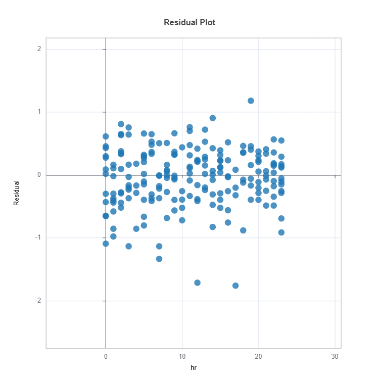
For the full list of arguments of the API see TestSuite.diagnose_residual_analysis.

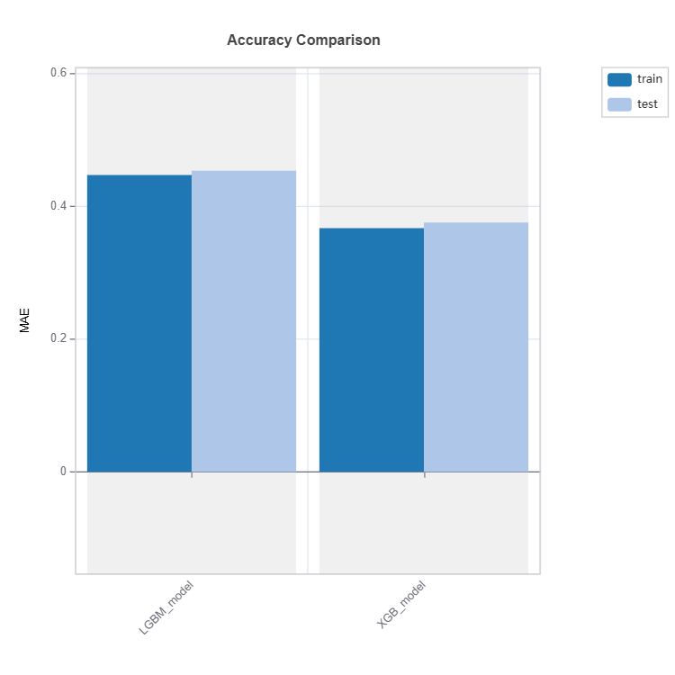
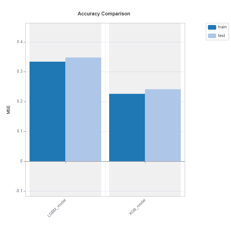
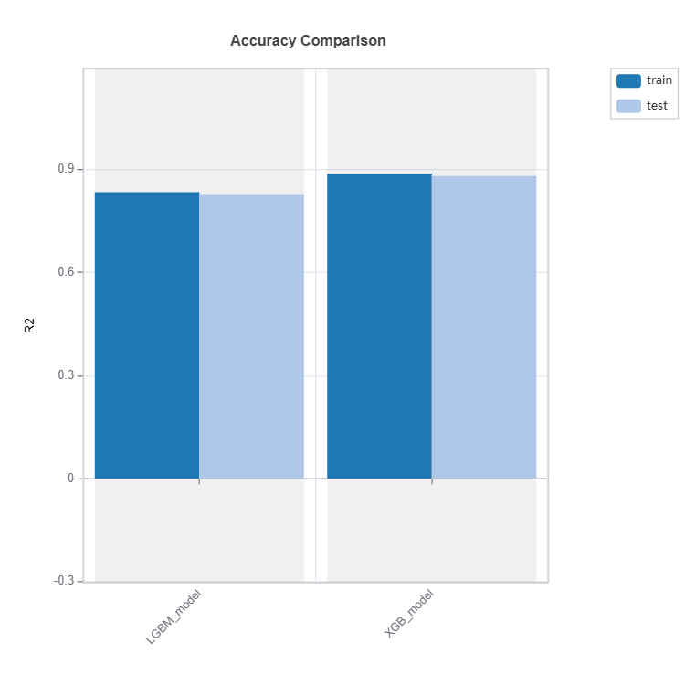
Performance Comparison#

Performance of several models can be compared as follows:

tsc = TestSuite(ds, models=[model_lgbm, model_xgb])
# Performance comparison of 2 models specified in tsc
results = tsc.compare_accuracy_table(train_dataset="train", test_dataset="test",
                                  metric=("MAE", "MSE", "R2"))
results.plot()

../../../_images/Accuracy_Comparison_MSE.png

../../../_images/Accuracy_Comparison_MAE.png

../../../_images/Accuracy_Comparison_R2.png

Check the API reference for detail arguments of TestSuite.compare_accuracy_table.

Supervised Learning for Residual Analysis#

MoDeVa provides supervised machine learning approach to analyze residuals, using interpretable gradient-boosted decision trees (GBDT) with depth-1 and depth-2 constraints and random forest (RF) proximity matrices for clustering. This methodology enhances model performance by identifying regions where the errors (e.g., mean absolute error (MAE) is high), enabling targeted interventions to refine predictive accuracy.

Traditional unsupervised approaches, such as binning, clustering (e.g., $k$-means), or decision tree-based methods, often fail to capture complex, non-linear relationships in high-dimensional feature spaces. Instead, GBDT and RF provide a supervised framework that explicitly models residual errors, leveraging ensemble learning to better capture feature interactions and high-error regions.

The interpretable GBDT model enables detailed feature analysis, identifying key variables and their effects on residuals. This makes it possible to pinpoint why and where errors are occurring in the feature space. Additionally, the RF proximity matrix offers a data-driven clustering mechanism by measuring pairwise similarity between data points based on their shared leaf memberships across trees. This proximity-based clustering aligns naturally with the underlying model behavior, making the results more interpretable and actionable compared to traditional clustering approaches.

By combining error-focused modeling, feature importance analysis, and proximity-based clustering, this framework provides a structured way to detect high-error regions. This enables targeted feature engineering, model refinement, and localized adjustments, ultimately improving overall model reliability and robustness.

Methodology#

There are two complementary methodologies available in MoDeVa:

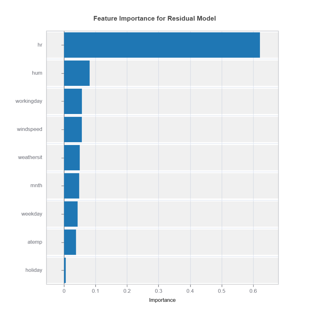
1. Residual Modeling Using Interpretable GBDT

We train an interpretable XGBoost model constrained to depth-1 and depth-2 trees, allowing us to explicitly model residuals.

The residuals $(r = | y - \hat{y} |)$ are used as the target variable in a separate regression model, where features explain where and why errors occur.

The depth constraint ensures that only direct feature effects (depth-1) and simple interactions (depth-2) are captured, making results interpretable.

Feature importance scores and effect from fANOVAare analyzed to understand which variables drive residuals the most.

results = ts.diagnose_residual_interpret(dataset='test', n_estimators=100, max_depth=2) # train interpretable GBDT model with depth-2
results.plot("feature_importance") # plot feature importance
results.plot("effect_importance") # plot effect importance

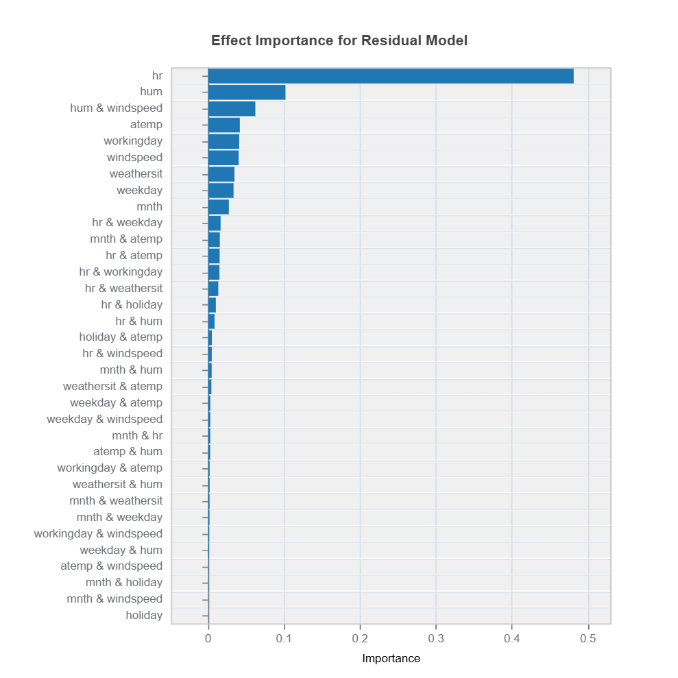
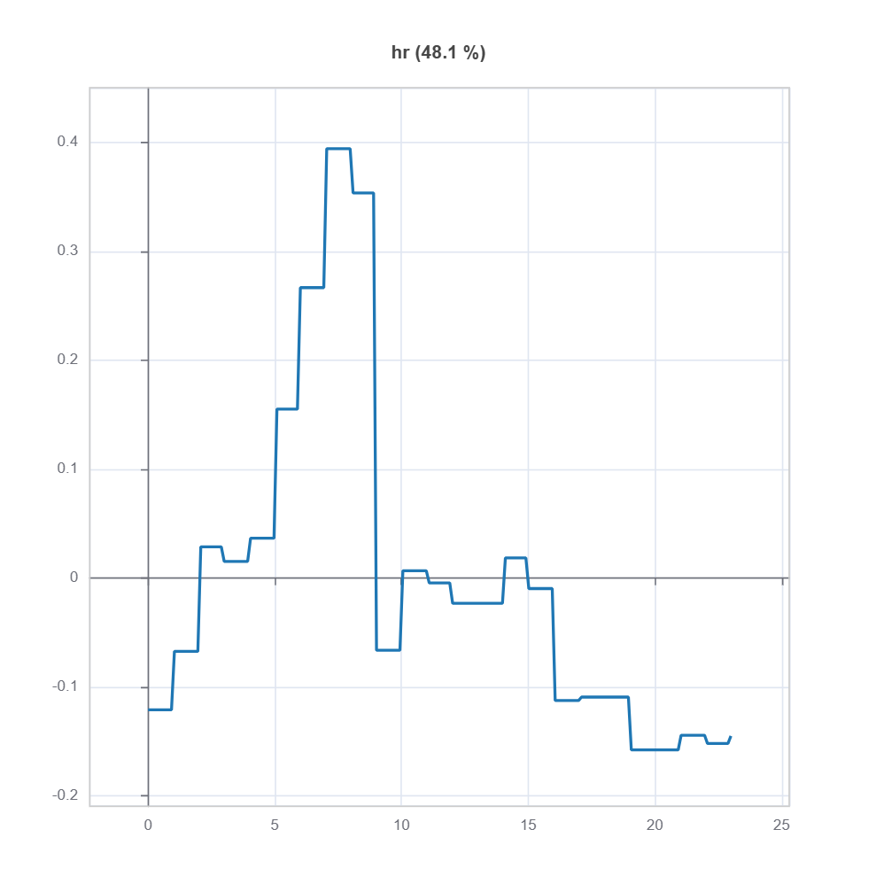
../../../_images/Feature_Importance_XGB_Residual_Model.png

../../../_images/Effect_Importance_XGB_Residual_Model.png

The effect plot of feature of to the residual model is shown below:

ts_residual = results.value["TestSuite"] # get the testsuite object
ts_residual.interpret_effects("hr", dataset="test").plot() # plot effect plot for feature "hr"

../../../_images/Effect_XGB_Residual_hr.png

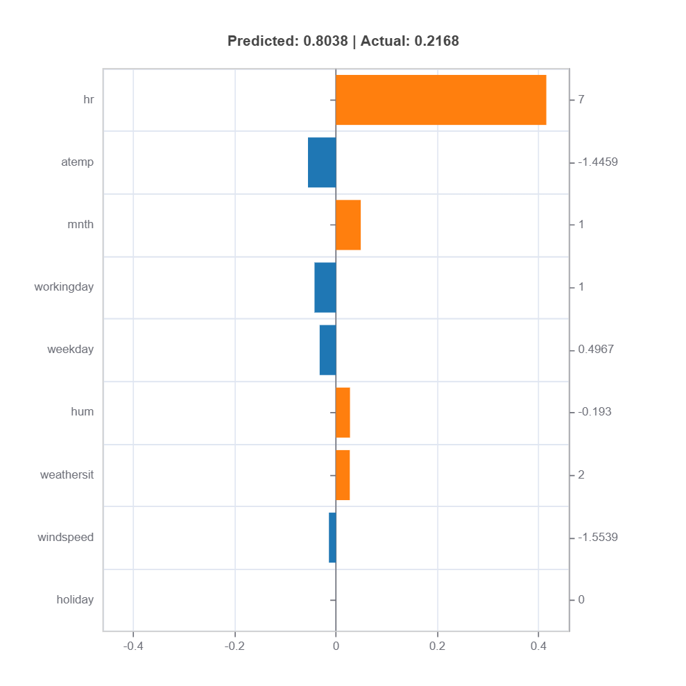
To understand the local effect for a sample, we can use the following code:

ts_residual.interpret_local_fi(sample_index=20).plot() # plot local feature importance for sample index 20

../../../_images/Local_FI_XGB_Residual_Model.png

2. Proximity-Based Clustering Using RF Proximity Matrix

A random forest model is trained on the same dataset, and the proximity matrix is extracted.

The proximity matrix measures pairwise similarity between data points by counting how often two points land in the same leaf across multiple trees.

This matrix is then used as an input to clustering algorithms, such as spectral clustering or hierarchical clustering, to group samples based on error similarity.

Unlike traditional clustering methods, this approach aligns clusters with the model’s behavior, making it more meaningful for residual error analysis.

MoDeVa code’s for this methodology is as follows:

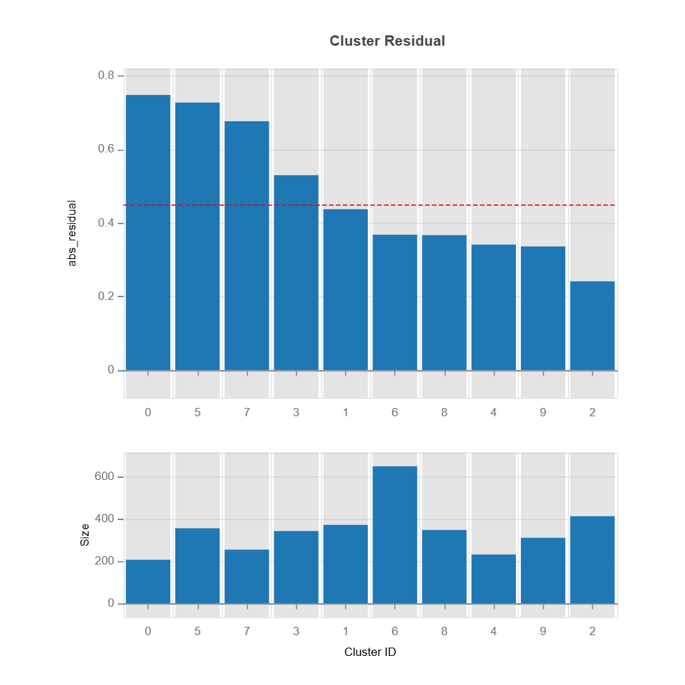
results = ts.diagnose_residual_cluster(
   dataset="test", # dataset to use
   response_type="abs_residual", # response type
   metric="MAE", # metric to use
   n_clusters=10, # number of clusters
   cluster_method="pam", # clustering method
   sample_size=2000, # sample size
   rf_n_estimators=100, # number of trees
   rf_max_depth=5, # max depth of trees
)
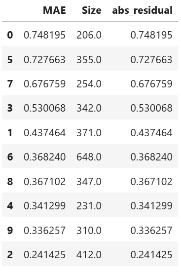
results.table # table of cluster performance
results.plot("cluster_residual")
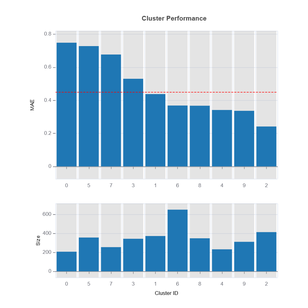
results.plot("cluster_performance")
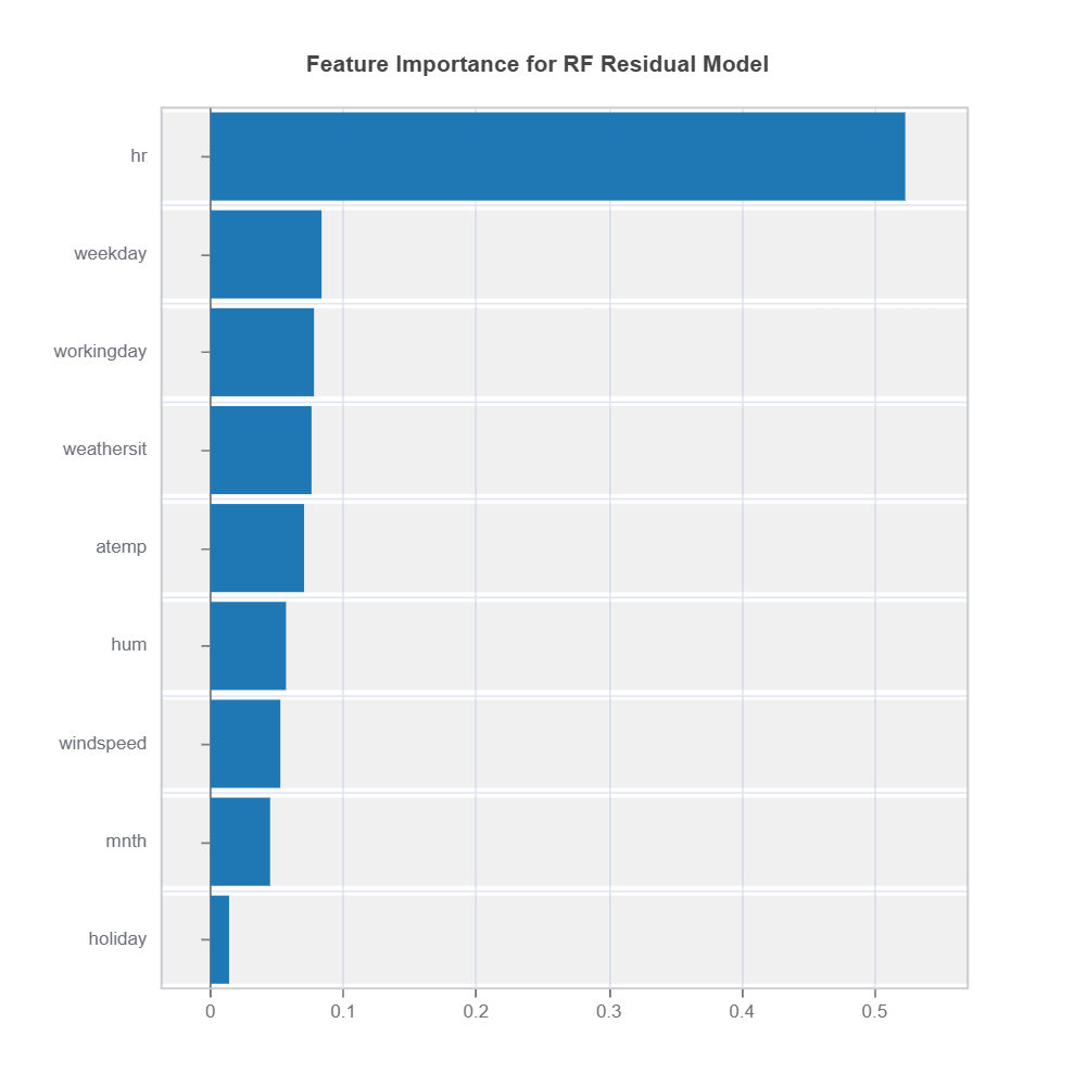
results.plot("feature_importance")

../../../_images/Cluster_Residual_Performance.png

../../../_images/Feature_Importance_RF_Residual.png

High-Error Region Identification and Interpretation

Clusters are analyzed based on their average residual error (e.g., MAE or MSE).

High-error clusters are interpreted based on their feature composition, helping to uncover systematic model weaknesses.

By leveraging GBDT feature importance and RF-based similarity, we gain insights into how feature interactions contribute to residuals.

Actionable interventions, such as feature transformations, localized model adjustments, or targeted data augmentation, are then developed to mitigate errors in identified high-error regions.

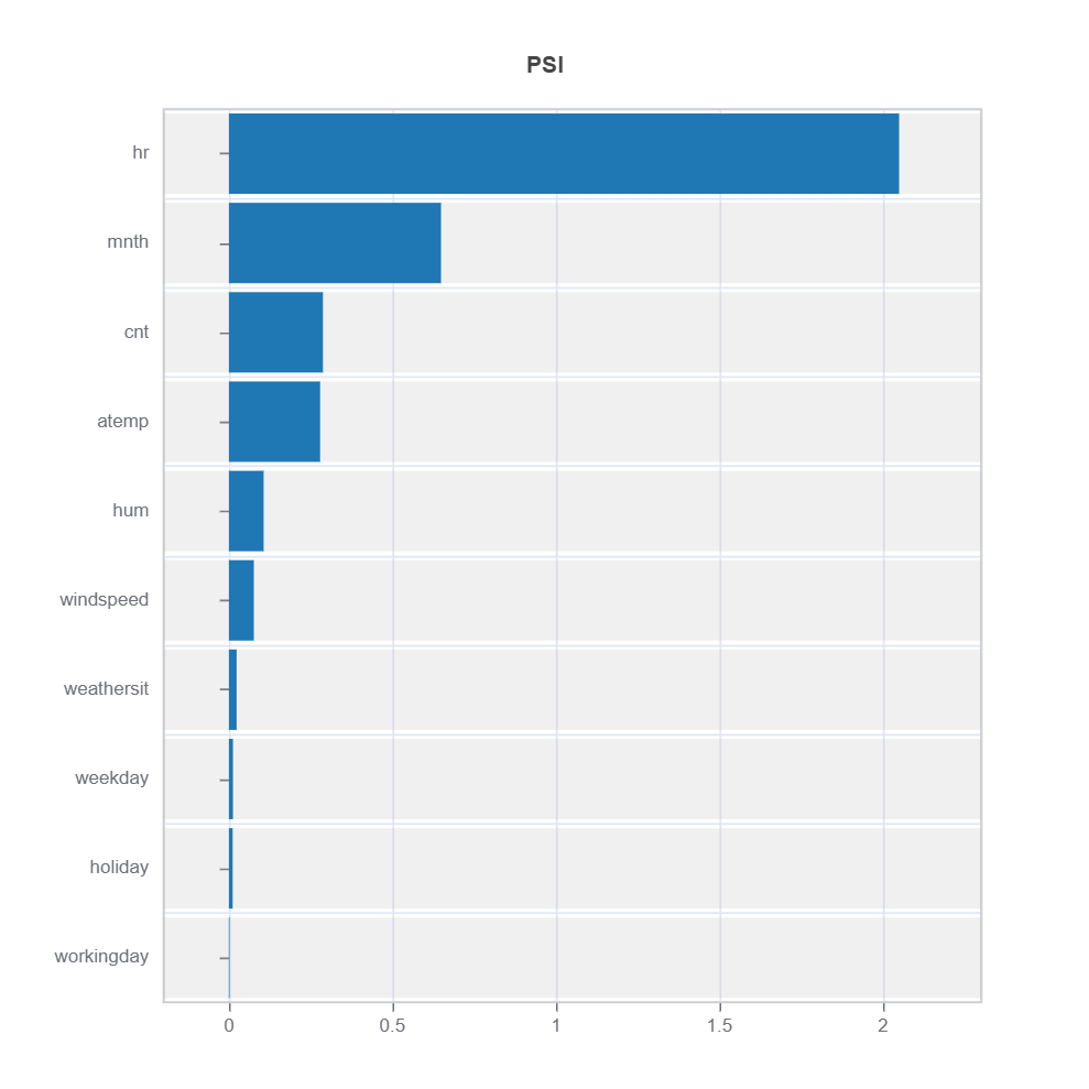
The following code shows how to identify the high-error region and interpret the results:

cluster_id = 2 # cluster id
data_results = ds.data_drift_test(
   **results.value["clusters"][cluster_id]["data_info"], # use the cluster_id
   distance_metric="PSI", # distance metric using PSI
   psi_method="uniform", # psi method using uniform distribution
   psi_bins=10 # psi bins
)
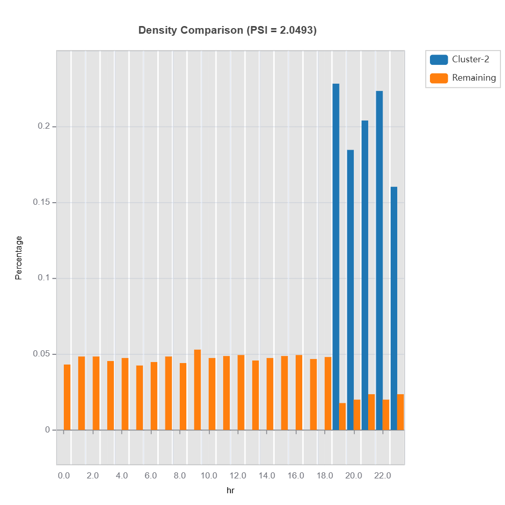
data_results.plot("summary") # plot summary of data drift test
data_results.plot(name=('density', 'hr')) # plot density plot for feature "hr"

../../../_images/Residual_Density_hr.png