Reliability

Reliability in predictive models refers to their ability to produce consistent and trustworthy outputs. Model reliability measures the confidence in a model’s predictions by identifying areas of high uncertainty and ensuring consistency over time. This is particularly important in high-stakes domains like banking, where unreliable predictions can lead to significant risks or losses.

Output uncertainty, or lack of confidence in predictions, arises from factors such as noisy data, sparse samples, or inherent model limitations.

Investigating and Improving Model Reliability

In MoDeVa, investigating and improving model reliability involves the following steps:

1. Uncertainty Quantification: Conformal Prediction (CP) is used to generate prediction intervals, providing a range within which the true value is likely to fall with a specified confidence level.

2. Identification of Less Reliable Regions: Model weakness identification involves pinpointing areas in the data where the model performs poorly or lacks confidence. In MoDeVa, this is achieved by examining two key factors: (1) High uncertainty regions and (2) Outside Conformal Prediction coverage.

3. Determine Impactful Variables: Identify key variables whose contribute to output uncertainty.

4. Enhance the Model: Address the identified issues by refining the model, such as through further analysis, introducing segment-specific models, or other tailored adjustments.

Conformal Prediction

Conformal prediction provides a model-agnostic framework for constructing prediction intervals with guaranteed coverage under minimal assumptions. The key idea is to quantify how different a new test point is from the training data using a nonconformity score.

The framework offers finite-sample, distribution-free coverage guarantees requiring only that the data are exchangeable. For a desired miscoverage rate α, conformal prediction produces prediction intervals that contain the true value with probability 1-α.

Full Conformal Prediction

Full conformal prediction requires refitting the model for each test point, making it computationally expensive.

Mathematical Formulation:

For a dataset \({(X_,Y_),...,(X_n,Y_n)}\) and test point \(X_{n+1}\):

\[C_{n,\alpha}(X_{n+1}) = \{y: \pi_y \geq \alpha\}\]

where:

• \(\pi_y\) is the p-value for candidate y

• For each \(y\), refit model on \({(X_,Y_),...,(X_n,Y_n),(X_{n+1},y)}\)

• Compute nonconformity scores and compare to calibration set

To reduce the computational burden, an approximate approach is used at the expense of reduction of coverage guarantee.

Split Conformal Prediction

Split conformal reduces computational cost by splitting data into proper training and calibration sets.

Algorithm:

1. Split data into training \(D_{\text{train}}\) and calibration \(D_{\text{cal}}\) sets

2. Train model on \(D_{\text{train}}\)

3. Compute nonconformity scores on \(D_{\text{cal}}\)

4. Use empirical quantiles of scores to construct prediction intervals

Binary Classification

For binary classification, nonconformity scores typically use predicted probabilities.

Nonconformity Score:

\[\begin{split}s_i = \begin{cases} 1 - \hat{p}_i & \text{if } y_i = 1 \\ \hat{p}_i & \text{if } y_i = 0 \end{cases}\end{split}\]

where:

• \(\hat{p}_i\) is predicted probability for class 1

• Lower scores indicate better conformity with training data

Conformalized Residual Quantile Regression (CRQR)

CRQR applies quantile regression to the residuals to estimate prediction intervals.

Algorithm

1. Base Model Fitting:

First, fit a base model \(f(X)\) to estimate conditional mean:

\[\hat{f}(X) = \mathbb{E}[Y|X]\]

Calculate residuals:

\[r_i = y_i - \hat{f}(x_i)\]

2. Residual Quantile Regression:

Train quantile regression on residuals for desired quantiles \(\tau_1\), \(\tau_2\):

\[\hat{q}_{\tau}(X) = \text{QR}_{\tau}(r|X)\]

3. Conformalization:

Compute nonconformity scores on calibration set:

\[s_i = \max\{\hat{q}_{\tau_1}(X_i) - r_i, r_i - \hat{q}_{\tau_2}(X_i)\}\]

4. Prediction Intervals:

For new point \(X\), construct interval:

\[C_{n,\alpha}(X) = \hat{f}(X) + [\hat{q}_{\tau_1}(X) - Q_{1-\alpha}(s), \hat{q}_{\tau_2}(X) + Q_{1-\alpha}(s)]\]

where:

• \(\hat{f}(X)\) is base model prediction

• \(\hat{q}_{τ}(X)\) are predicted residual quantiles

• \(Q_{1-α}(s)\) is (1-α) quantile of calibration scores

Advantages and Considerations

1. Distribution-free coverage guarantees

2. Works with any base predictor

3. Split conformal trades statistical efficiency for computational efficiency

4. Residual approach can capture heteroscedasticity

5. Can be extended to handle covariate shift

Reliability Analysis in MoDeVa

Data Setup

from modeva import DataSet
# Create dataset object holder
ds = DataSet()
# Loading MoDeVa pre-loaded dataset "Bikesharing"
ds.load(name="BikeSharing")  # Changed dataset name
## Preprocess the data
ds.scale_numerical(features=("cnt",), method="log1p") # Log transfomed target
ds.set_feature_type(feature="hr", feature_type="categorical") # set to categorical feature
ds.set_feature_type(feature="mnth", feature_type="categorical")
ds.scale_numerical(features=ds.feature_names_numerical, method="standardize") # standardized numerical features
ds.set_inactive_features(features=("yr", "season", "temp")) # deactivate some features
ds.preprocess()
## Split data into training and testing sets randomly
ds.set_random_split()

Model Setup

# Regression tasks using lightGBM and xgboost
from modeva.models import MoLGBMRegressor, MoXGBRegressor

# for lightGBM
model_lgbm = MoLGBMRegressor(name = "LGBM_model", max_depth=2, n_estimators=100)
# for xgboost
model_xgb = MoXGBRegressor(name = "XGB_model", max_depth=2, n_estimators=100)

Model Training

# train model with input: ds.train_x and target: ds.train_y
model_lgbm.fit(ds.train_x, ds.train_y)
model_xgb.fit(ds.train_x, ds.train_y)

Reporting and Diagnostic Setup

# Create a testsuite that bundles dataset and model
from modeva import TestSuite
ts = TestSuite(ds, model_lgbm) # store bundle of dataset and model in fs

Reliability Assessment:

In the example of regression task below, split conformal prediction is used.

• Expected coverage of prediction intervals, \(\alpha\) = 0.1

• Test dataset is split into:

  • 50% of data is used to train Quantile regression using LightGBM with tree depth 5 for the residuals and calibration

  • 50% of data and testing

# reliability assessment using Split Conformal Prediction
results = ts.diagnose_reliability(
    train_dataset="test", # train dataset
    test_dataset="test",
    test_size=0.5,
    alpha=0.1,
    max_depth=5,
    random_state=0)
results.table

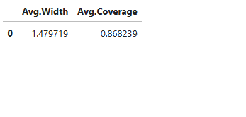
The table shows the average width of prediction interval and the coverage.

For the full list of arguments of the API see TestSuite.diagnose_reliability.

Identification of Reliability Issue and Impactful Variables

There are several ways to identify reliability issues (finding region in the input space with high uncertainty): * Apply slicing technique to identify variables and their intervals with less reliable outputs * Fit inherently interpretable model (e.g., xgboost depth-2) with prediction reliability (or in our out coverage) as target and plot the effects (main or interaction) as well as variable importance with respected to reliability measure. * Select sub-samples with less reliable outputs and visualize and compare the distributions between unreliable vs. the rest. Distribution difference can be quantified using measure such as PSI.

Less reliable outputs can be identified by analyzing two key aspects of conformal prediction outputs:

1. High Uncertainty

2. Out-of-Coverage Instances

For Regression:

Measure prediction interval width:

\[W(X) = q_{\tau_2}(X) + Q_{1-\alpha}(s) - (q_{\tau_1}(X) - Q_{1-\alpha}(s))\]

Flag points where:

\[W(X) \gt Q_{1-\beta}(W)\]

where:

• \(\beta\) is threshold (e.g., 0.9 for top 10% widest intervals)

• \(Q_1₋\beta(W)\) is the \((1-\beta)\) quantile of interval widths

For Binary Classification:

Flag instances where:

\[|C_{n,\alpha}(X)| \in \{0, 2\}\]

where:

• \(|C_{n,\alpha}(X)|\) = 0: Empty prediction set (high uncertainty)

• \(|C_{n,\alpha}(X)|\) = 2: Both classes predicted (high uncertainty)

1. Coverage Violation Detection:

For true value \(y\) and prediction set \(C_{n,\alpha}(X)\):

\[V(X,y) = \mathbb{1}\{y \notin C_{n,\alpha}(X)\}\]

2. Region Characterization:

Analyze feature distributions where:

\[P(V(X,y) = 1 | X \in R) \gt \alpha\]

where:

• \(R\) is a region in feature space

• \(\alpha\) is nominal miscoverage rate

Common patterns indicating model weakness:

• High uncertainty + good coverage: Model is honest about uncertainty

• High uncertainty + poor coverage: Model may be misspecified

• Low uncertainty + poor coverage: Model is overconfident

Reliability Diagnostics in MoDeVa

To understand the region with higher uncertainty can be analyzed as follows:

data_results = ds.data_drift_test(
    **results.value["data_info"],
    distance_metric="PSI",
    psi_method="uniform",
    psi_bins=10)

The results of distribution between less reliable region vs. overal data from TestSuite.diagnose_reliability is evaluated using DataSet.data_drift_test

• Percent of worst sample = 0.1 (10%) is selected for least reliable

• Metrics: PSI with 10 uniform binning is used for calculation.

data_results.plot() displays the following results:

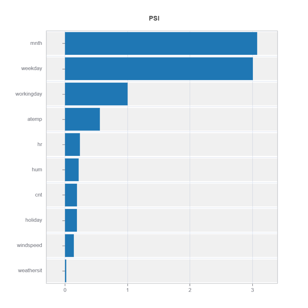
• Summary of distribution differences for all the features ranked by PSI

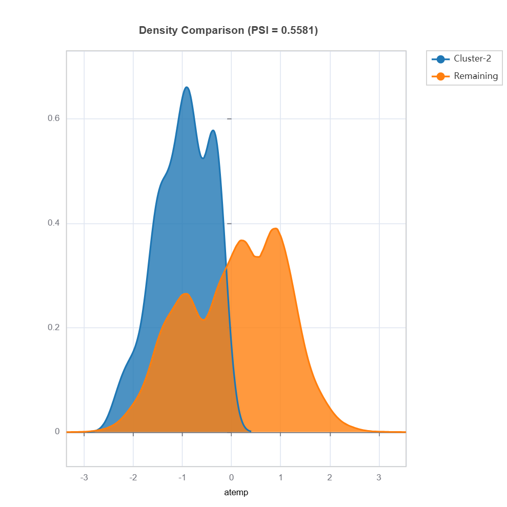
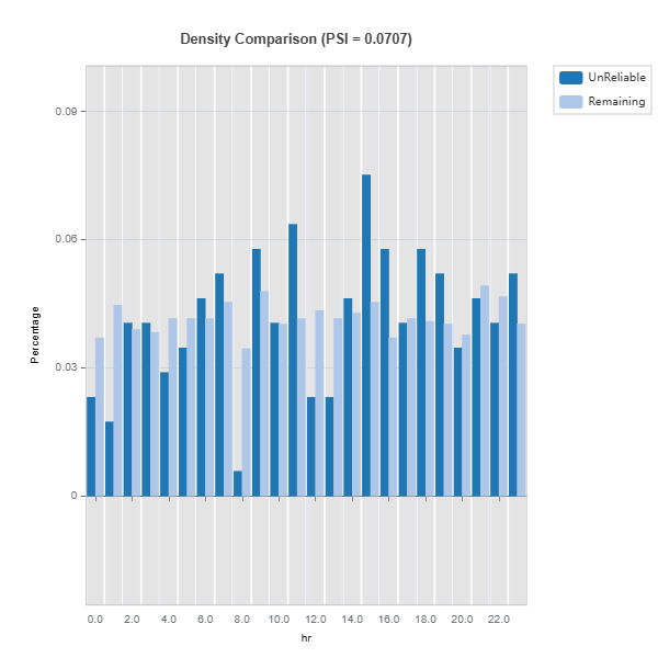
• Marginal density comparison of distribution shift

• Marginal histogram comparison of distribution shift

Summary of variable ranked according to their PSI (distribution difference)

data_results.plot("summary")

Plot the density of variables: To understand the distribution of unreliable region vs. the remaining, marginal distribution plot can be used as follows.

data_results.plot(("density", "hr"))

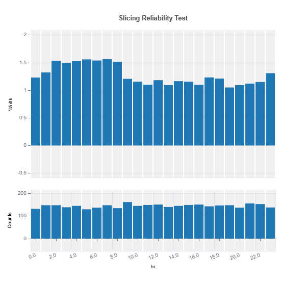
Slicing Reliability The reliability for a given feature can be analyzed through feature slicing. Below is an example for features=”hr” and metric=”width”:

results = ts.diagnose_slicing_reliability(
    features="hr",
    train_dataset="train",
    test_dataset="test",
    test_size=0.5,
    metric="width",
    random_state=0)
results.plot()

For the full list of arguments of the API see TestSuite.diagnose_slicing_reliability.

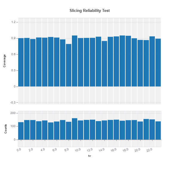
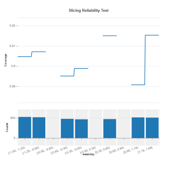
Univariate slicing for multiple features

results = ts.diagnose_slicing_reliability(
    features=(("hr",), ("atemp",), ("weekday",)),
    train_dataset="train",
    test_dataset="test",
    test_size=0.5,
    metric="coverage",
    random_state=0)
results.plot("hr")
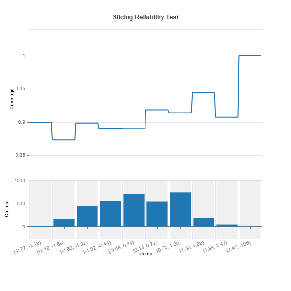
results.plot("atemp")
results.plot("weekday")

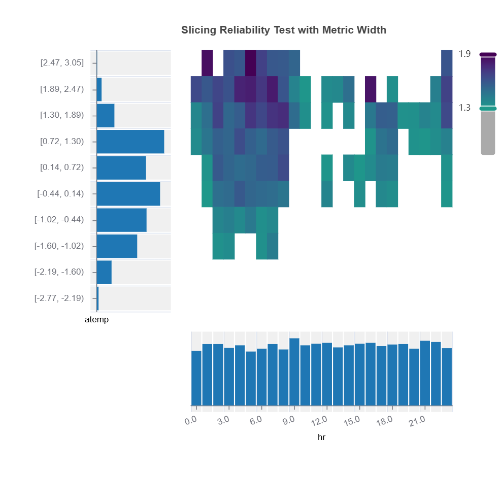
Bivariate slicing: interactions on reliability

results = ts.diagnose_slicing_reliability(
    features=("hr", "atemp"),
    train_dataset="train",
    test_dataset="test",
    test_size=0.5,
    random_state=0)
results.plot()

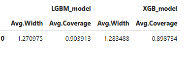
Reliability Comparison

Reliability of several models can be compared as follows:

fsc = TestSuite(ds, models=[model_lgbm, model_xgb])
# resilreliability comparison of 2 models specified in fsc
 results = fsc.compare_reliability(
     train_dataset="train",
     test_dataset="test",
     test_size=0.5,
     alpha=0.1,
     max_depth=5,
     random_state=0
 )
 results.table

Check the API reference for detail arguments of TestSuite.compare_reliability.

The uncertainty of multiple models can be compared for each feature using variable slicing:

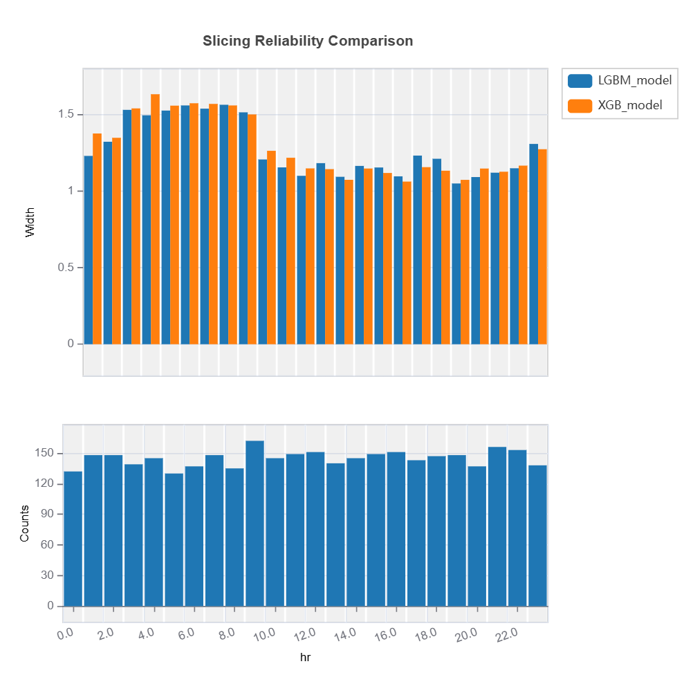
Check the API reference for detail arguments of TestSuite.compare_slicing_reliability.

Strategies for Addressing Model Weaknesses

Data-Centric Approaches

1. Targeted Data Augmentation:

For regions with high uncertainty or poor coverage:

\[R_{weak} = \{X: W(X) > Q_{1-β}(W) \text{ or } V(X,y) = 1\}\]

Solutions:

• Collect additional samples in \(R_{\text{weak}}\)

• Active learning in high-uncertainty regions

2. Feature Engineering:

Based on weakness patterns:

• Create interaction terms for regions with nonlinear patterns

• Develop domain-specific features where coverage is poor

• Transform features where uncertainty is heterogeneous

1. Local Model Enhancement:

For identified weak regions \(R_{\text{weak}}\):

\[\begin{split}f_{enhanced}(X) = \begin{cases} f_{local}(X) & \text{if } X \in R_{weak} \\ f_{global}(X) & \text{otherwise} \end{cases}\end{split}\]

Strategies:

• Train specialized models for \(R_{\text{weak}}\) (segmentation)

• Ensemble models with region-specific weights (Mixture of Experts)

2. Architecture Modifications:

Based on uncertainty patterns:

• Add capacity in high-uncertainty regions or use alternative modeling framework

• Incorporate domain knowledge via constraints

• Use mixture of experts for heterogeneous regions

3. Loss Function Adjustments:

\[L_{new}(X,y) = L_{original}(X,y) + \lambda W(X)R(X)\]

where:

• \(R(X)\) is an indicator for weak regions

• \(\lambda\) balances overall performance vs local improvement

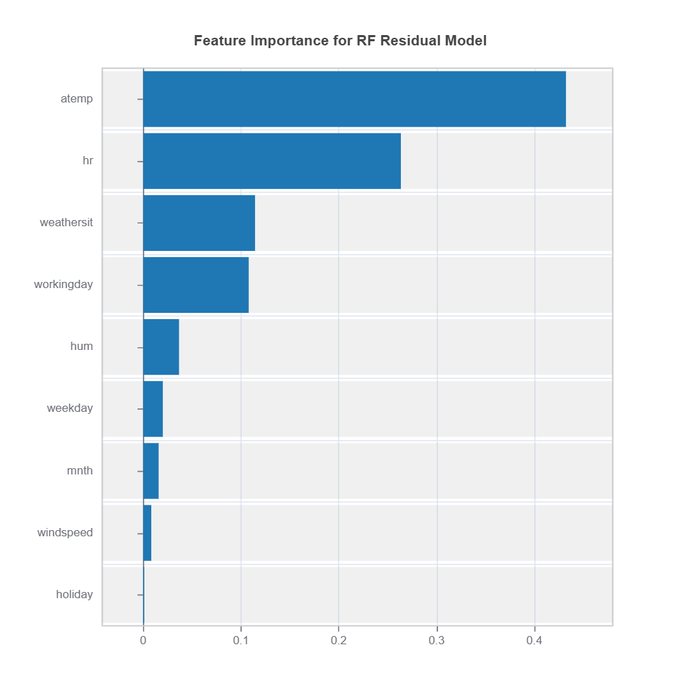
Supervised Machine Learning: Random Forest Clustering

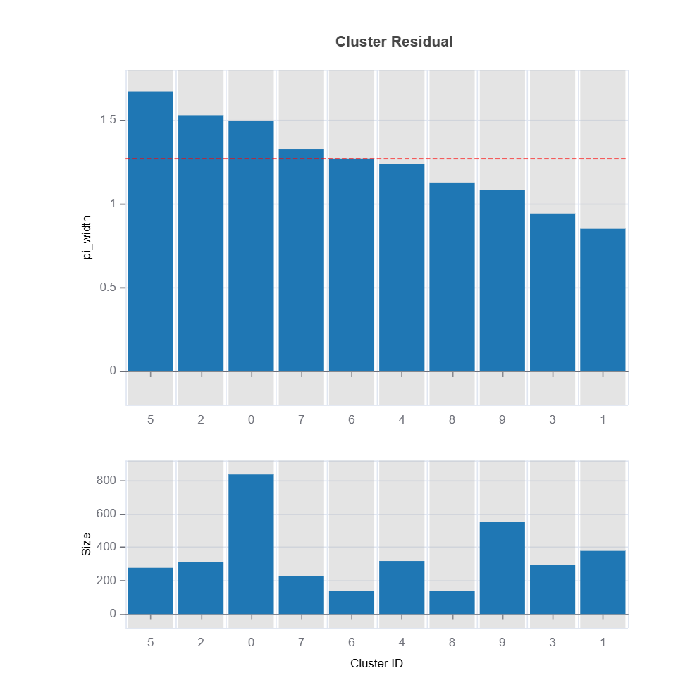
Prediction interval width can be used as a target clustering variable for supervised machine learning clustering using Random Forest proximity..

results = ts.diagnose_residual_cluster(
    dataset="test", # dataset
    response_type="pi_width", # response type
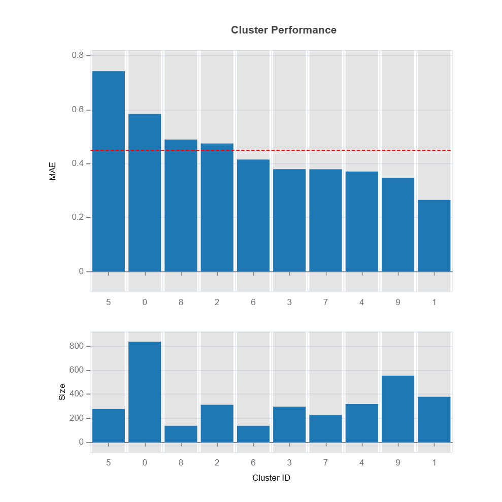
    metric="MAE", # metric
    n_clusters=10, # number of clusters
    cluster_method="pam", # clustering method
    sample_size=2000, # sample size
    rf_n_estimators=100, # number of trees
rf_max_depth=5,
)
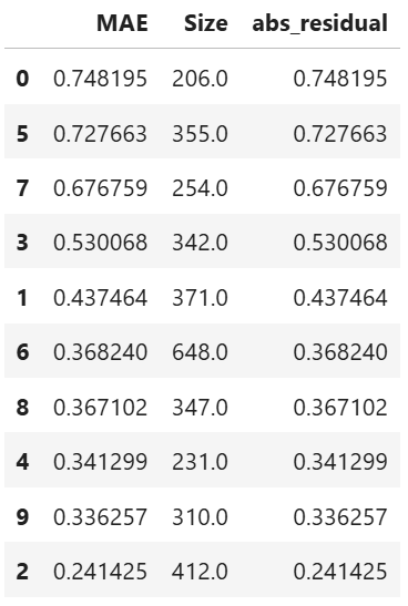
results.table #
results.plot() #

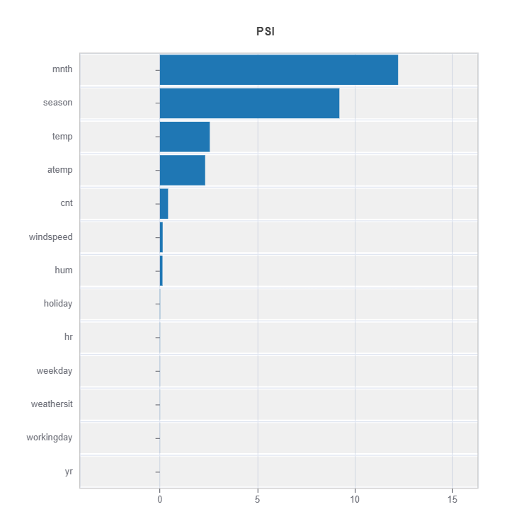
The following code shows how to identify the high-uncertainty region and interpret the results:

cluster_id = 2 # cluster id
data_results = ds.data_drift_test(
   **results.value["clusters"][cluster_id]["data_info"], # use the cluster_id
   distance_metric="PSI", # distance metric using PSI
   psi_method="uniform", # psi method using uniform distribution
   psi_bins=10 # psi bins
)
data_results.plot("summary") # plot summary of data drift test
data_results.plot(name=('density', 'atemp')) # plot density plot for feature "hr"

Examples

Example 1: Bike Sharing

The example below demonstrates how to use MoDeVa with its high-code APis for the Bike Sharing dataset from the UCI repository, which consists of 20,640 samples and 9 features, fetched by sklearn.datasets. The response variable MedHouseVal (Median Home Value) is continuous and is a regression problem.

• Reliability Analysis (Regression)

Examples 2: Taiwan Credit

The second example below demonstrates how to use MoDeVa’s high-code APIs for the TaiwanCredit dataset from the UCI repository. This dataset comprises the credit card details of 30,000 clients in Taiwan from April 2005 to September 2005, and more information can be found on the TaiwanCreditData website. The FlagDefault variable serves as the response for this classification problem.

• Reliability Analysis (Classification)