Weakness Detection

Weakness detection in predictive machine learning models is the process of identifying areas in the input space where the model underperforms or makes incorrect predictions. These regions are often characterized by high residual errors, poor predictions, or patterns of bias. Effective weakness detection improves model reliability, robustness, and fairness, ensuring it performs well across all data segments.

Introduction

Why Weakness Detection is Important

1. Improve Model Performance: - Identify areas where the model struggles and refine it through targeted improvements.

2. Enhance Trustworthiness: - Address systematic biases or recurring errors to build confidence in the model.

3. Guide Data Collection: - Pinpoint areas where additional data can enhance model performance.

4. Mitigate Risks: - Detect and address weaknesses before deploying the model in production.

Key Approaches to Weakness Detection

1. Residual Analysis: - Examine prediction errors to uncover regions with systematic weaknesses.

2. Data Slicing: - Divide the dataset into smaller subsets to evaluate localized performance.

3. Feature Sensitivity: - Identify features or feature interactions linked to poor predictions.

4. Visualization: - Use plots and metrics to locate weak regions in the feature space.

Weakness Detection in MoDeVa

Data Setup

from modeva import DataSet
# Create dataset object holder
ds = DataSet()
# Loading MoDeVa pre-loaded dataset "TaiwanCredit"
ds = DataSet(name="TaiwanCredit")
ds.load("TaiwanCredit")
# Encode categorical data into ordinal
ds.encode_categorical(method="ordinal")
# Execute data pre-processing
ds.preprocess()
# Set target variable
ds.set_target("FlagDefault")
# Set the following variables as inactive (not used for modeling)
ds.set_inactive_features(["SEX", "MARRIAGE", "AGE"])
# Randomly split training and testing set
ds.set_random_split()

Model Setup

# Classification tasks using lightGBM and xgboost
from modeva.models import MoLGBMClassifier, MoXGBClassifier

# for lightGBM
model_lgbm = MoLGBMClassifier(name = "LGBM_model", max_depth=2, n_estimators=100)
# for xgboost
model_xgb = MoXGBClassifier(name = "XGB_model", max_depth=2, n_estimators=100)

Model Training

# train model with input: ds.train_x and target: ds.train_y
model_lgbm.fit(ds.train_x, ds.train_y)
model_xgb.fit(ds.train_x, ds.train_y)

Reporting and Diagnostic Setup

# Create a testsuite that bundles dataset and model
from modeva import TestSuite
ts = TestSuite(ds, model_lgbm) # store bundle of dataset and model in fs
# Evaluate performance and summarize into table
results = ts.diagnose_accuracy_table(train_dataset="train", test_dataset="test")
results.table
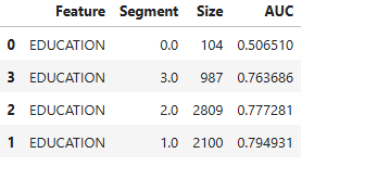
# Slicing categorical feature
results = ts.diagnose_slicing_accuracy(features="EDUCATION", metric="AUC",
                                   threshold=0.65)
results.table

For the full list of arguments of the API see TestSuite.diagnose_accuracy_table and TestSuite.diagnose_slicing_accuracy.

Error Slicing for Weakness Detection

Slicing data into bins is a common technique for identifying model weaknesses. Binning divides a feature into segments to assess model performance in specific regions. Below are three popular binning methods: uniform binning, quantile binning, and automatic binning using a depth-1 XGBoost tree.

1. Uniform Binning

Uniform binning divides a feature’s range into equal-sized intervals, regardless of the data distribution.

How It Works:

1. Identify the minimum and maximum values of the feature.

2. Divide the range into equally spaced bins.

3. Assign each data point to its corresponding bin.

Advantages:

• Simple and easy to interpret.

• Works well with uniformly distributed features.

Disadvantages:

• Can result in empty or sparse bins for skewed distributions.

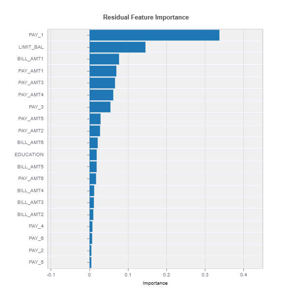
Example in MoDeVa: The following is an example to identify feature importance driving the error.

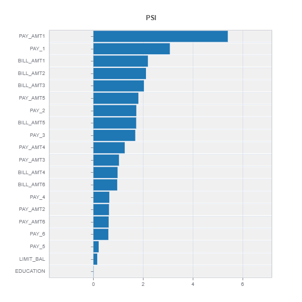
# Analyze residual feature importance
results = ts.diagnose_residual_fi(method="uniform")
results.plot()

For the full list of arguments of the API see `TestSuite.diagnose_accuracy_residual_fi`_.

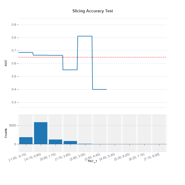
# Uniform binning numerical feature
results = ts.diagnose_slicing_accuracy(features=(("LIMIT_BAL", ), ("PAY_1", )),
                                   method="uniform",
                                   bins=10, metric="AUC",
                                   threshold=0.65)
results.plot()

For the full list of arguments of the API see TestSuite.diagnose_slicing_accuracy.

2. Quantile Binning

Quantile binning divides the feature range such that each bin contains approximately the same number of samples.

How It Works:

1. Compute quantiles based on the desired number of bins.

2. Assign each data point to a bin based on its quantile.

Advantages:

• Handles skewed distributions effectively.

• Ensures equal representation in bins.

Disadvantages:

• Bin widths may vary, complicating interpretation.

• Sensitive to outliers.

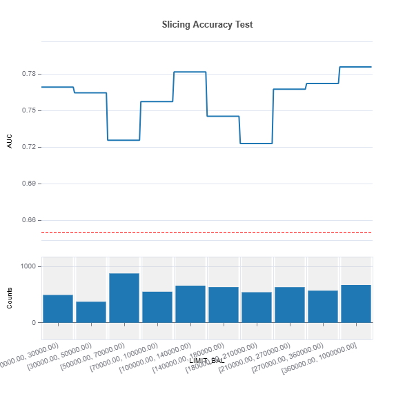
Example in MoDeVa:

# Quantile binning
results = ts.diagnose_slicing_accuracy(features="LIMIT_BAL",
                                   method="quantile",
                                   bins=10, metric="AUC",
                                   threshold=0.65)
results.plot()

3. Automatic Binning Using a Depth-1 or 2 XGBoost Tree

This method uses a depth-1 or 2 XGBoost tree to automatically determine the optimal split point for a feature based on its relationship with the target. Use variable importance statistics and visualization to understand variables driving errors.

How It Works:

1. Train a depth-1 or 2 XGBoost tree using the feature and target variable.

2. Extract the tree’s split point.

3. Divide the feature values into bins based on the split.

Advantages:

• Automatically identifies bins optimized for target performance.

• Captures meaningful splits based on the feature-target relationship.

Disadvantages:

• May result in uneven bin distribution.

• Relies on the model’s ability to identify meaningful splits.

Example in MoDeVa:

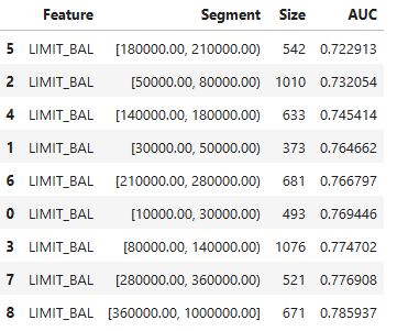
# Automatic binning
results = ts.diagnose_slicing_accuracy(features="LIMIT_BAL",
                                   method="auto-xgb1",
                                   bins=10,
                                   metric="AUC",
                                   threshold=0.75)
results.plot()  # Display results in plot
results.table   # Display results in table

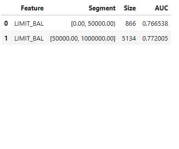
User-defined Binning:

# Customm binning
results = ts.diagnose_slicing_accuracy(features="LIMIT_BAL", method="precompute",
                                   bins={"LIMIT_BAL": (0.0, 50000, 1000000)},
                                   metric="AUC")
results.table   # Display results in table

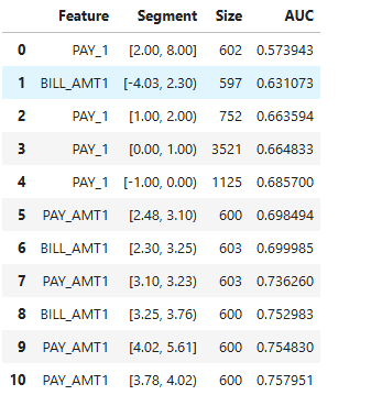
Slicing for a Set of Features:

results = ts.diagnose_slicing_accuracy(features=(("PAY_1", ), ("BILL_AMT1",), ("PAY_AMT1", )),
                                   method="quantile", metric="AUC", threshold=0.6)
results.table

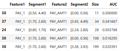
2-Feature Interaction Slicing:

results = ts.diagnose_slicing_accuracy(features=("PAY_1", "PAY_AMT1"),
                                   method="uniform", bins=10,
                                   metric="AUC", threshold=0.5)
results.table

Slicing data through binning allows for detailed weakness detection by isolating feature ranges or regions where the model performs poorly. Uniform and quantile binning are simple yet effective for exploratory analysis, while automatic binning using a depth-1 XGBoost tree provides optimized, target-driven insights. These methods, when combined, offer a robust framework for identifying and addressing model weaknesses.

Additional Utilities for Slicing

Retrieving samples below threshold value

from modeva.testsuite.utils.slicing_utils import get_data_info
data_info = get_data_info(res_value=results.value)[("PAY_1", "PAY_AMT1")]
data_info

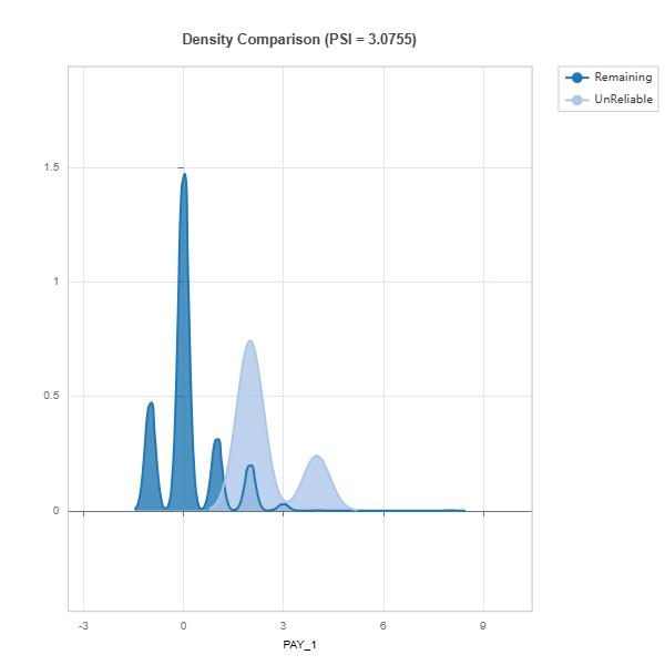
Testing distribution difference between weak samples and the rest

data_results = ds.data_drift_test(**data_info, distance_metric="PSI",
                              psi_method="uniform", psi_bins=10)
data_results.plot("summary")

# To get the list of figure names in the "data_results" object for further plotting
data_results.get_figure_names()

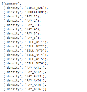
# Example of plotting from the list of figures
data_results.plot(('density', 'PAY_1'))

Weakness Comparison

Slices of several models can be compared as follows:

1. Numerical Features

tsc = TestSuite(ds, models=[model_lgbm, model_xgb])
results = tsc.compare_slicing_accuracy(features="PAY_AMT1", method="quantile",
                                   bins=10, metric="AUC")
results.plot()

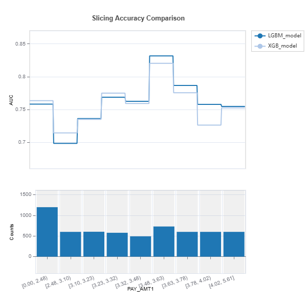
Check the API reference for detail arguments of TestSuite.compare_slicing_accuracy.

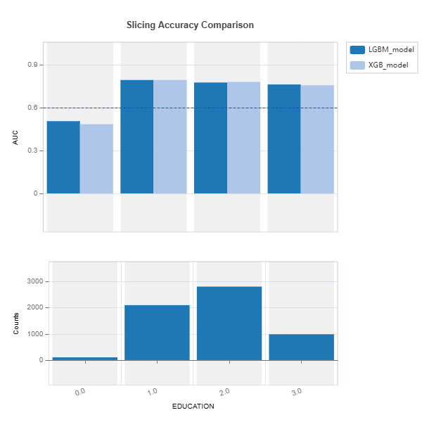
2. Categorical Features

tsc = TestSuite(ds, models=[model1, model2])
results = tsc.compare_slicing_accuracy(features="EDUCATION", metric="AUC",
                                   threshold=0.6)
results.plot()

Advanced Slicing

Advanced slicing techniques can be used to detect and analyze model weaknesses in terms of robustness, reliability, and resilience. By dividing the data into meaningful subsets, practitioners can systematically evaluate the model’s behavior under varying conditions and identify specific areas where performance degrades.

1. Robustness: Sensitivity to Noisy Inputs

Robustness measures a model’s ability to maintain performance when subjected to input perturbations or noise. Advanced slicing can help detect regions where the model is overly sensitive. The detail description of the robustness test can be found in the robustness testing section.

2. Reliability: Uncertainty of Predictions

Reliability focuses on understanding where the model’s predictions are uncertain. Slicing can highlight regions with high uncertainty, revealing where predictions lack confidence. The detail description of the reliability test can be found in the reliability testing section.

3. Resilience: Performance Heterogeneity and Distribution Drift

Resilience measures how well a model performs under distribution shifts and across heterogeneous data subsets. Slicing helps detect regions of poor performance or changes in data distribution. The detail description of the resilience test can be found in the resilience testing section.

Examples

Example 1: Bike Sharing

The example below demonstrates how to use MoDeVa with its high-code APis for the Bike Sharing dataset from the UCI repository, which consists of 20,640 samples and 9 features, fetched by sklearn.datasets. The response variable MedHouseVal (Median Home Value) is continuous and is a regression problem.

• Sliced Performance (Regression)

Examples 2: Taiwan Credit

The second example below demonstrates how to use MoDeVa’s high-code APIs for the TaiwanCredit dataset from the UCI repository. This dataset comprises the credit card details of 30,000 clients in Taiwan from April 2005 to September 2005, and more information can be found on the TaiwanCreditData website. The FlagDefault variable serves as the response for this classification problem.

• Sliced Performance (Classification)